Pytorch Intro: Everything you want to know

Pytorch 本质是和python完全不一样的东西。然后这东西本质是拿来训练模型的，其他的事情它干的一般般的。

学习链接

官方教程
Welcome to PyTorch Tutorials — PyTorch Tutorials 2.7.0+cu126 documentation
Learning PyTorch with Examples — PyTorch Tutorials 2.7.0+cu126 documentation
他人的教程
【深度学习】60题PyTorch简易入门指南，做技术的弄潮儿 - 知乎

数据集导入

MNIST

import torch
from torch import nn
from torch.utils.data import DataLoader
from torchvision import datasets
from torchvision.transforms import ToTensor

# 导入
# Download training data from open datasets.
training_data = datasets.FashionMNIST(
    root="data",
    train=True,
    download=True,
    transform=ToTensor(),
)

# Download test data from open datasets.
test_data = datasets.FashionMNIST(
    root="data",
    train=False,
    download=True,
    transform=ToTensor(),
)

# Create data loaders.
train_dataloader = DataLoader(training_data, batch_size=batch_size)
test_dataloader = DataLoader(test_data, batch_size=batch_size)

for X, y in test_dataloader:
    print(f"Shape of X [N, C, H, W]: {X.shape}")
    print(f"Shape of y: {y.shape} {y.dtype}")
    break

CIFAR10

trainset = torchvision.datasets.CIFAR10(root='../data', train=True, download=True, transform=transform_train)
trainloader = torch.utils.data.DataLoader(trainset, batch_size=BATCH_SIZE, shuffle=True, num_workers=2)

testset = torchvision.datasets.CIFAR10(root='../data', train=False, download=True, transform=transform_test)
testloader = torch.utils.data.DataLoader(testset, batch_size=100, shuffle=False, num_workers=2)

可视化+预处理

其实我们大部分的工作都是在这个层面做，所以听起来很蠢。

Datasets & DataLoaders — PyTorch Tutorials 2.7.0+cu126 documentation

import torch
from torch.utils.data import Dataset
from torchvision import datasets
from torchvision.transforms import ToTensor
import matplotlib.pyplot as plt

training_data = datasets.FashionMNIST(
    root="data",
    train=True,
    download=True,
    transform=ToTensor()
)

test_data = datasets.FashionMNIST(
    root="data",
    train=False,
    download=True,
    transform=ToTensor()
)

labels_map = {
    0: "T-Shirt",
    1: "Trouser",
    2: "Pullover",
    3: "Dress",
    4: "Coat",
    5: "Sandal",
    6: "Shirt",
    7: "Sneaker",
    8: "Bag",
    9: "Ankle Boot",
}
figure = plt.figure(figsize=(8, 8))
cols, rows = 3, 3
for i in range(1, cols * rows + 1):
    sample_idx = torch.randint(len(training_data), size=(1,)).item()
    img, label = training_data[sample_idx]
    figure.add_subplot(rows, cols, i)
    plt.title(labels_map[label])
    plt.axis("off")
    plt.imshow(img.squeeze(), cmap="gray")
plt.show()

ToTensordata

ToTensor converts a PIL image or NumPy ndarray into a FloatTensor. and scales the image’s pixel intensity values in the range[0.,1.]

Lambda Transforms

Lambda transforms apply any user-defined lambda function. Here, we define a function to turn the integer into a one-hot encoded tensor. It first creates a zero tensor of size 10 (the number of labels in our dataset) and calls scatter_ which assigns a value=1 on the index as given by the label y.

target_transform = Lambda(lambda y: torch.zeros(
    10, dtype=torch.float).scatter_(dim=0, index=torch.tensor(y), value=1))

Tensorboard

Visualizing Models, Data, and Training with TensorBoard — PyTorch Tutorials 2.7.0+cu126 documentation

In the 60 Minute Blitz, we show you how to load in data, feed it through a model we define as a subclass of nn.Module, train this model on training data, and test it on test data. To see what’s happening, we print out some statistics as the model is training to get a sense for whether training is progressing. However, we can do much better than that: PyTorch integrates with TensorBoard, a tool designed for visualizing the results of neural network training runs. This tutorial illustrates some of its functionality, using the Fashion-MNIST dataset which can be read into PyTorch using torchvision.datasets.

Tensor 张量

Tensors — PyTorch Tutorials 2.7.0+cu126 documentation

from torch.utils.tensorboard import SummaryWriter

# default `log_dir` is "runs" - we'll be more specific here
writer = SummaryWriter('runs/fashion_mnist_experiment_1')

# get some random training images
dataiter = iter(trainloader)
images, labels = next(dataiter)

# create grid of images
img_grid = torchvision.utils.make_grid(images)

# show images
matplotlib_imshow(img_grid, one_channel=True)

# write to tensorboard
writer.add_image('four_fashion_mnist_images', img_grid)

tensorboard --logdir=runs

Projector!

# helper function
def select_n_random(data, labels, n=100):
    '''
    Selects n random datapoints and their corresponding labels from a dataset
    '''
    assert len(data) == len(labels)

    perm = torch.randperm(len(data))
    return data[perm][:n], labels[perm][:n]

# select random images and their target indices
images, labels = select_n_random(trainset.data, trainset.targets)

# get the class labels for each image
class_labels = [classes[lab] for lab in labels]

# log embeddings
features = images.view(-1, 28 * 28)
writer.add_embedding(features,
                    metadata=class_labels,
                    label_img=images.unsqueeze(1))
writer.close()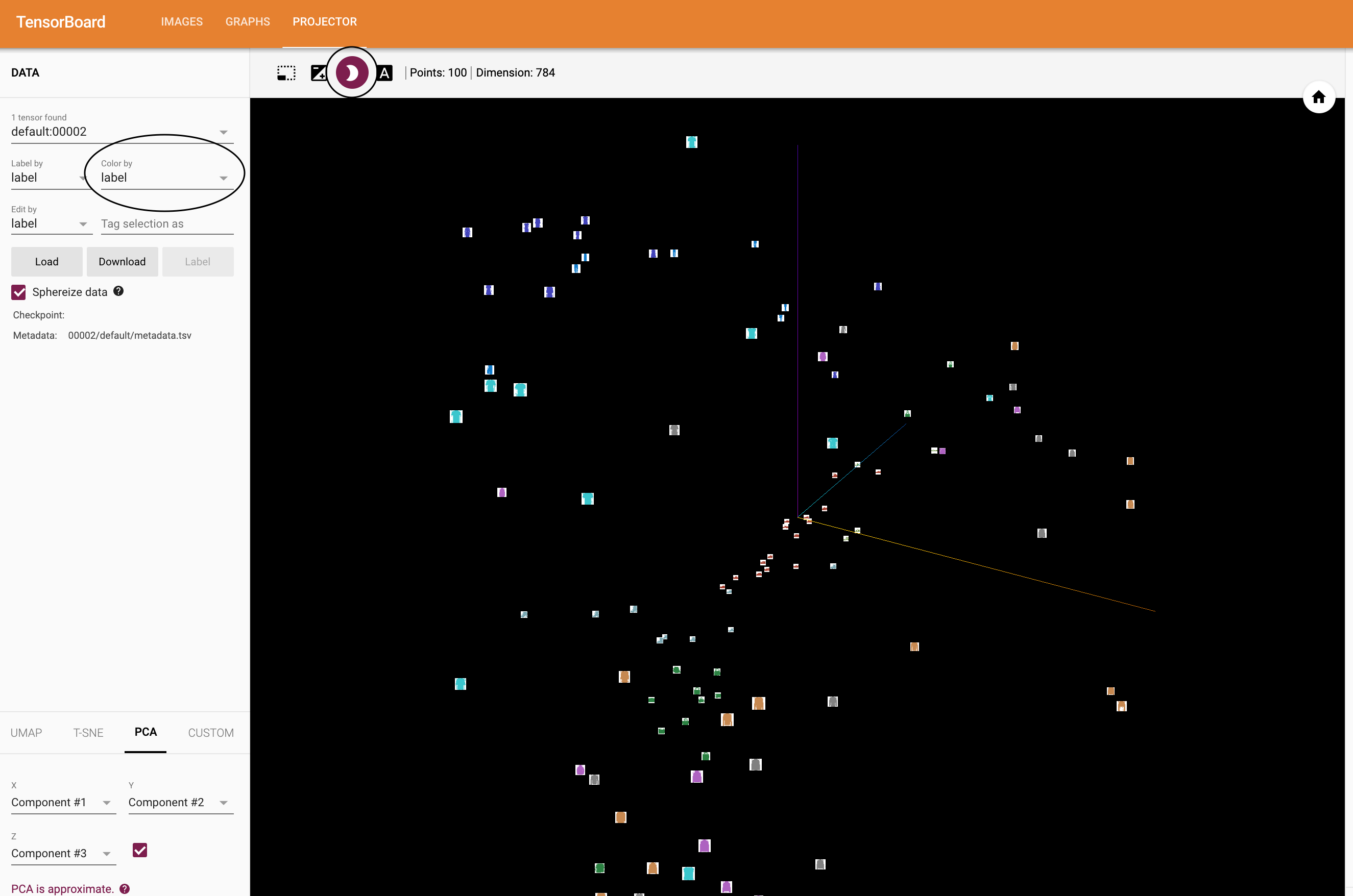

tracking

# helper functions

def images_to_probs(net, images):
    '''
    Generates predictions and corresponding probabilities from a trained
    network and a list of images
    '''
    output = net(images)
    # convert output probabilities to predicted class
    _, preds_tensor = torch.max(output, 1)
    preds = np.squeeze(preds_tensor.numpy())
    return preds, [F.softmax(el, dim=0)[i].item() for i, el in zip(preds, output)]

def plot_classes_preds(net, images, labels):
    '''
    Generates matplotlib Figure using a trained network, along with images
    and labels from a batch, that shows the network's top prediction along
    with its probability, alongside the actual label, coloring this
    information based on whether the prediction was correct or not.
    Uses the "images_to_probs" function.
    '''
    preds, probs = images_to_probs(net, images)
    # plot the images in the batch, along with predicted and true labels
    fig = plt.figure(figsize=(12, 48))
    for idx in np.arange(4):
        ax = fig.add_subplot(1, 4, idx+1, xticks=[], yticks=[])
        matplotlib_imshow(images[idx], one_channel=True)
        ax.set_title("{0}, {1:.1f}%\n(label: {2})".format(
            classes[preds[idx]],
            probs[idx] * 100.0,
            classes[labels[idx]]),
                    color=("green" if preds[idx]==labels[idx].item() else "red"))
    return fig

running_loss = 0.0
for epoch in range(1):  # loop over the dataset multiple times

    for i, data in enumerate(trainloader, 0):

        # get the inputs; data is a list of [inputs, labels]
        inputs, labels = data

        # zero the parameter gradients
        optimizer.zero_grad()

        # forward + backward + optimize
        outputs = net(inputs)
        loss = criterion(outputs, labels)
        loss.backward()
        optimizer.step()

        running_loss += loss.item()
        if i % 1000 == 999:    # every 1000 mini-batches...

            # ...log the running loss
            writer.add_scalar('training loss',
                            running_loss / 1000,
                            epoch * len(trainloader) + i)

            # ...log a Matplotlib Figure showing the model's predictions on a
            # random mini-batch
            writer.add_figure('predictions vs. actuals',
                            plot_classes_preds(net, inputs, labels),
                            global_step=epoch * len(trainloader) + i)
            running_loss = 0.0
print('Finished Training')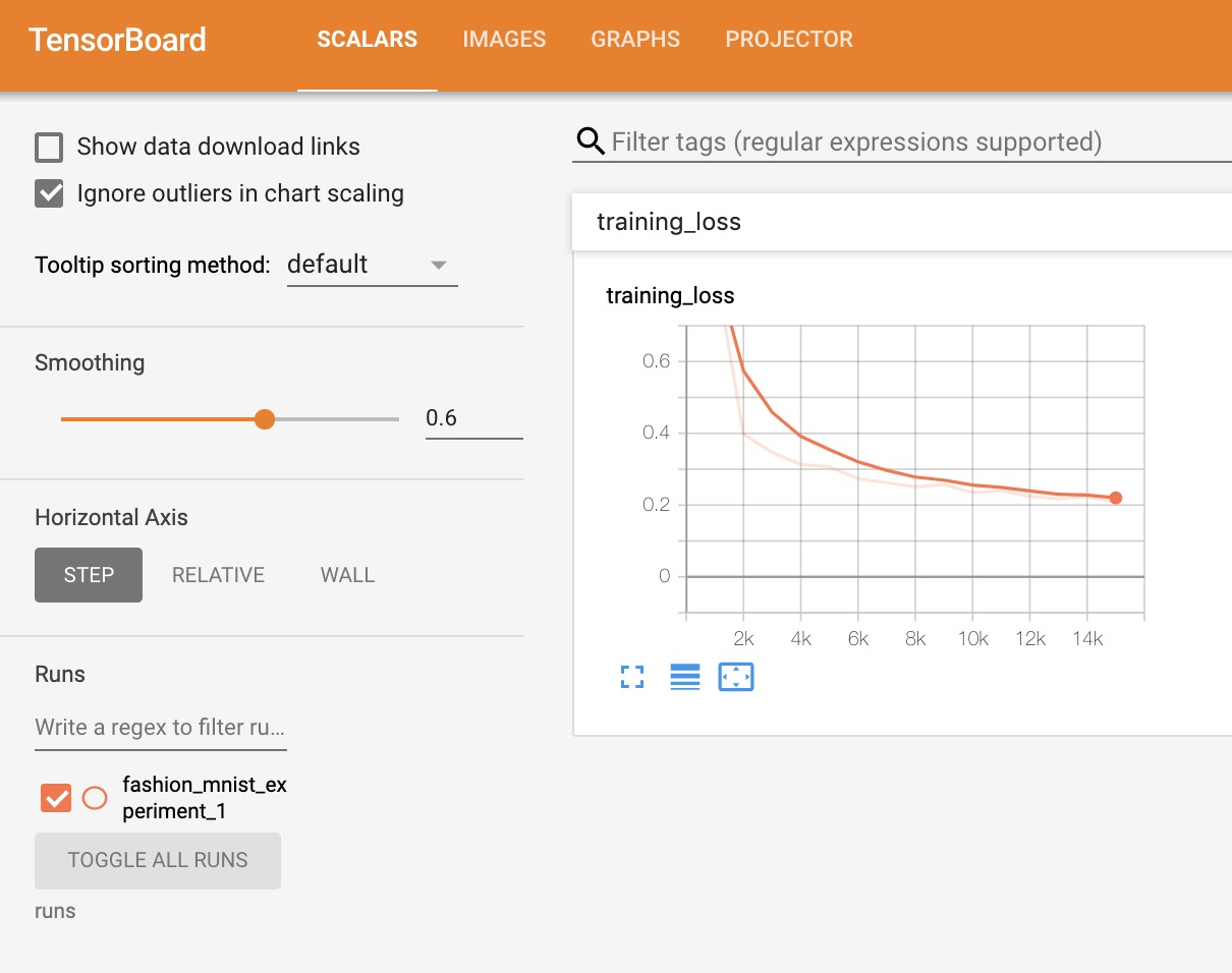

学习张量

Hello, Tensor!

import torch
import numpy as np

# 1. init from num
data = [[1, 2],[3, 4]]
x_data = torch.tensor(data)

# 2. init from numpy
np_array = np.array(data)
x_np = torch.from_numpy(np_array)

# 3. another tensor
x_ones = torch.ones_like(x_data) # retains the properties of x_data
print(f"Ones Tensor: \n {x_ones} \n")

x_rand = torch.rand_like(x_data, dtype=torch.float) # overrides the datatype of x_data
print(f"Random Tensor: \n {x_rand} \n")

# 4. Random
shape = (2,3,)
rand_tensor = torch.rand(shape)
ones_tensor = torch.ones(shape)
zeros_tensor = torch.zeros(shape)

print(f"Random Tensor: \n {rand_tensor} \n")
print(f"Ones Tensor: \n {ones_tensor} \n")
print(f"Zeros Tensor: \n {zeros_tensor}")

Tensor 的内部var

形状等

tensor = torch.rand(3,4)

print(f"Shape of tensor: {tensor.shape}")
print(f"Datatype of tensor: {tensor.dtype}")
print(f"Device tensor is stored on: {tensor.device}")

有1200个算子供君选择：torch — PyTorch 2.7 documentation
Over 1200 tensor operations, including arithmetic, linear algebra, matrix manipulation (transposing, indexing, slicing), sampling and more are comprehensively described here.

合并张量：

t1 = torch.cat([tensor, tensor, tensor], dim=1)
print(t1)

计算

# This computes the matrix multiplication between two tensors. y1, y2, y3 will have the same value
# ``tensor.T`` returns the transpose of a tensor
y1 = tensor @ tensor.T
y2 = tensor.matmul(tensor.T)

y3 = torch.rand_like(y1)
torch.matmul(tensor, tensor.T, out=y3)

# This computes the element-wise product. z1, z2, z3 will have the same value
z1 = tensor * tensor
z2 = tensor.mul(tensor)

z3 = torch.rand_like(tensor)
torch.mul(tensor, tensor, out=z3)

Single-element tensors If you have a one-element tensor, for example by aggregating all values of a tensor into one value, you can convert it to a Python numerical value using item():

agg = tensor.sum()
agg_item = agg.item()
print(agg_item, type(agg_item))

In-place operations Operations that store the result into the operand are called in-place. They are denoted by a _ suffix. For example: x.copy_(y), x.t_(), will change x.

print(f"{tensor} \n")
tensor.add_(5)
print(tensor)

tensor([[1., 0., 1., 1.],
        [1., 0., 1., 1.],
        [1., 0., 1., 1.],
        [1., 0., 1., 1.]])

tensor([[6., 5., 6., 6.],
        [6., 5., 6., 6.],
        [6., 5., 6., 6.],
        [6., 5., 6., 6.]])

Tensors on the CPU and NumPy arrays can share their underlying memory locations, and changing one will change the other

back to numpy

t = torch.ones(5)
print(f"t: {t}")
n = t.numpy()
print(f"n: {n}")

t: tensor([1., 1., 1., 1., 1.])
n: [1. 1. 1. 1. 1.]

t.add_(1)
print(f"t: {t}")
print(f"n: {n}")

t: tensor([2., 2., 2., 2., 2.])
n: [2. 2. 2. 2. 2.]

array to tensor

n = np.ones(5)
t = torch.from_numpy(n)

np.add(n, 1, out=n)
print(f"t: {t}")
print(f"n: {n}")

t: tensor([2., 2., 2., 2., 2.], dtype=torch.float64)
n: [2. 2. 2. 2. 2.]

神经网络层

Build the Neural Network — PyTorch Tutorials 2.7.0+cu126 documentation

NLP models & layers
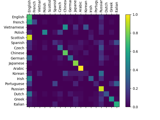
NLP from Scratch — PyTorch Tutorials 2.7.0+cu126 documentation

import os
import torch
from torch import nn
from torch.utils.data import DataLoader
from torchvision import datasets, transforms

device = torch.accelerator.current_accelerator().type if torch.accelerator.is_available() else "cpu"
print(f"Using {device} device")

Define the class:

class NeuralNetwork(nn.Module):
    def __init__(self):
        super().__init__()
        self.flatten = nn.Flatten()
        self.linear_relu_stack = nn.Sequential(
            nn.Linear(28*28, 512),
            nn.ReLU(),
            nn.Linear(512, 512),
            nn.ReLU(),
            nn.Linear(512, 10),
        )

    def forward(self, x):
        x = self.flatten(x)
        logits = self.linear_relu_stack(x)
        return logits

model = NeuralNetwork().to(device)
print(model)

NeuralNetwork(
  (flatten): Flatten(start_dim=1, end_dim=-1)
  (linear_relu_stack): Sequential(
    (0): Linear(in_features=784, out_features=512, bias=True)
    (1): ReLU()
    (2): Linear(in_features=512, out_features=512, bias=True)
    (3): ReLU()
    (4): Linear(in_features=512, out_features=10, bias=True)
  )
)

X = torch.rand(1, 28, 28, device=device)
logits = model(X)
pred_probab = nn.Softmax(dim=1)(logits)
y_pred = pred_probab.argmax(1)
print(f"Predicted class: {y_pred}")

nn.Flatten

We initialize the nn.Flatten layer to convert each 2D 28x28 image into a contiguous array of 784 pixel values ( the minibatch dimension (at dim=0) is maintained).

flatten = nn.Flatten()
flat_image = flatten(input_image)
print(flat_image.size())

nn.Linear

The linear layer is a module that applies a linear transformation on the input using its stored weights and biases.

layer1 = nn.Linear(in_features=28*28, out_features=20)
hidden1 = layer1(flat_image)
print(hidden1.size())

nn.ReLU

Non-linear activations are what create the complex mappings between the model’s inputs and outputs. They are applied after linear transformations to introduce nonlinearity, helping neural networks learn a wide variety of phenomena.
In this model, we use nn.ReLU between our linear layers, but there’s other activations to introduce non-linearity in your model.

print(f"Before ReLU: {hidden1}\n\n")
hidden1 = nn.ReLU()(hidden1)
print(f"After ReLU: {hidden1}")

nn.Sequential

nn.Sequential is an ordered container of modules. The data is passed through all the modules in the same order as defined. You can use sequential containers to put together a quick network like seq_modules.

seq_modules = nn.Sequential(
    flatten,
    layer1,
    nn.ReLU(),
    nn.Linear(20, 10)
)
input_image = torch.rand(3,28,28)
logits = seq_modules(input_image)

nn.Softmax

The last linear layer of the neural network returns logits - raw values in[-infty, infty] - which are passed to the nn.Softmax module. The logits are scaled to values [0, 1] representing the model’s predicted probabilities for each class. dim parameter indicates the dimension along which the values must sum to 1.

softmax = nn.Softmax(dim=1)
pred_probab = softmax(logits)

Model Params

Many layers inside a neural network are parameterized, i.e. have associated weights and biases that are optimized during training. Subclassing nn.Module automatically tracks all fields defined inside your model object, and makes all parameters accessible using your model’s parameters() or named_parameters() methods.

In this example, we iterate over each parameter, and print its size and a preview of its values.

print(f"Model structure: {model}\n\n")

for name, param in model.named_parameters():
    print(f"Layer: {name} | Size: {param.size()} | Values : {param[:2]} \n")

Model structure: NeuralNetwork(
  (flatten): Flatten(start_dim=1, end_dim=-1)
  (linear_relu_stack): Sequential(
    (0): Linear(in_features=784, out_features=512, bias=True)
    (1): ReLU()
    (2): Linear(in_features=512, out_features=512, bias=True)
    (3): ReLU()
    (4): Linear(in_features=512, out_features=10, bias=True)
  )
)

Layer: linear_relu_stack.0.weight | Size: torch.Size([512, 784]) | Values : tensor([[ 0.0234,  0.0034, -0.0202,  ..., -0.0088, -0.0105,  0.0194],
        [-0.0330,  0.0198,  0.0253,  ..., -0.0193,  0.0315,  0.0338]],
       device='cuda:0', grad_fn=<SliceBackward0>)

Layer: linear_relu_stack.0.bias | Size: torch.Size([512]) | Values : tensor([-0.0254,  0.0035], device='cuda:0', grad_fn=<SliceBackward0>)

Layer: linear_relu_stack.2.weight | Size: torch.Size([512, 512]) | Values : tensor([[-0.0382, -0.0342, -0.0422,  ...,  0.0037,  0.0401, -0.0393],
        [ 0.0317, -0.0257, -0.0345,  ..., -0.0333, -0.0069,  0.0142]],
       device='cuda:0', grad_fn=<SliceBackward0>)

Layer: linear_relu_stack.2.bias | Size: torch.Size([512]) | Values : tensor([-0.0265, -0.0096], device='cuda:0', grad_fn=<SliceBackward0>)

Layer: linear_relu_stack.4.weight | Size: torch.Size([10, 512]) | Values : tensor([[ 0.0208,  0.0163,  0.0114,  ...,  0.0172,  0.0008,  0.0140],
        [-0.0098, -0.0260, -0.0226,  ...,  0.0136,  0.0085,  0.0082]],
       device='cuda:0', grad_fn=<SliceBackward0>)

Layer: linear_relu_stack.4.bias | Size: torch.Size([10]) | Values : tensor([ 0.0129, -0.0352], device='cuda:0', grad_fn=<SliceBackward0>)

torch.nn — PyTorch 2.7 documentation

模型 Models

 we create a class that inherits from nn.Module. We define the layers of the network in the __init__ function and specify how data will pass through the network in the forward function. To accelerate operations in the neural network, we move it to the accelerator such as CUDA, MPS, MTIA, or XPU. If the current accelerator is available, we will use it. Otherwise, we use the CPU.
 

device = torch.accelerator.current_accelerator().type if torch.accelerator.is_available() else "cpu"
print(f"Using {device} device")

# Define model
class NeuralNetwork(nn.Module):
    def __init__(self):
        super().__init__()
        self.flatten = nn.Flatten()
        self.linear_relu_stack = nn.Sequential(
            nn.Linear(28*28, 512),
            nn.ReLU(),
            nn.Linear(512, 512),
            nn.ReLU(),
            nn.Linear(512, 10)
        )

    def forward(self, x):
        x = self.flatten(x)
        logits = self.linear_relu_stack(x)
        return logits

model = NeuralNetwork().to(device)  # init model and put it into device
print(model)

输出：

Using cuda device
NeuralNetwork(
  (flatten): Flatten(start_dim=1, end_dim=-1)
  (linear_relu_stack): Sequential(
    (0): Linear(in_features=784, out_features=512, bias=True)
    (1): ReLU()
    (2): Linear(in_features=512, out_features=512, bias=True)
    (3): ReLU()
    (4): Linear(in_features=512, out_features=10, bias=True)
  )
)

1. LeNet

import torch
import torch.nn as nn

class LeNet(nn.Module):
    def __init__(self):
        super(LeNet, self).__init__()
        self.conv_stack = nn.Sequential(
            nn.Conv2d(1, 6, kernel_size=5, stride=1, padding=2),  # 1x32x32 -> 6x28x28
            nn.ReLU(),
            nn.AvgPool2d(kernel_size=2, stride=2),  # 6x28x28 -> 6x14x14
            nn.Conv2d(6, 16, kernel_size=5, stride=1),  # 6x14x14 -> 16x10x10
            nn.ReLU(),
            nn.AvgPool2d(kernel_size=2, stride=2),  # 16x10x10 -> 16x5x5
        )
        self.fc_stack = nn.Sequential(
            nn.Flatten(),
            nn.Linear(16 * 5 * 5, 120),  # 16x5x5 = 400 -> 120
            nn.ReLU(),
            nn.Linear(120, 84),
            nn.ReLU(),
            nn.Linear(84, 10),  # 10 classes
        )

    def forward(self, x):
        x = self.conv_stack(x)
        logits = self.fc_stack(x)
        return logits

# Example usage
device = torch.device("cuda" if torch.cuda.is_available() else "cpu")
model = LeNet().to(device)
print(model)

import torch
import torch.nn as nn
import torch.nn.functional as F

class Net(nn.Module):

    def __init__(self):  # 这里要放有参数的层
        super(Net, self).__init__()
        # 1 input image channel, 6 output channels, 5x5 square convolution
        # kernel
        self.conv1 = nn.Conv2d(1, 6, 5)
        self.conv2 = nn.Conv2d(6, 16, 5)
        # an affine operation: y = Wx + b
        self.fc1 = nn.Linear(16 * 5 * 5, 120)  # 5*5 from image dimension
        self.fc2 = nn.Linear(120, 84)
        self.fc3 = nn.Linear(84, 10)

    def forward(self, input):  # 这里要放对参数操作的层
        # Convolution layer C1: 1 input image channel, 6 output channels,
        # 5x5 square convolution, it uses RELU activation function, and
        # outputs a Tensor with size (N, 6, 28, 28), where N is the size of the batch
        c1 = F.relu(self.conv1(input))
        # Subsampling layer S2: 2x2 grid, purely functional,
        # this layer does not have any parameter, and outputs a (N, 6, 14, 14) Tensor
        s2 = F.max_pool2d(c1, (2, 2))
        # Convolution layer C3: 6 input channels, 16 output channels,
        # 5x5 square convolution, it uses RELU activation function, and
        # outputs a (N, 16, 10, 10) Tensor
        c3 = F.relu(self.conv2(s2))
        # Subsampling layer S4: 2x2 grid, purely functional,
        # this layer does not have any parameter, and outputs a (N, 16, 5, 5) Tensor
        s4 = F.max_pool2d(c3, 2)
        # Flatten operation: purely functional, outputs a (N, 400) Tensor
        s4 = torch.flatten(s4, 1)
        # Fully connected layer F5: (N, 400) Tensor input,
        # and outputs a (N, 120) Tensor, it uses RELU activation function
        f5 = F.relu(self.fc1(s4))
        # Fully connected layer F6: (N, 120) Tensor input,
        # and outputs a (N, 84) Tensor, it uses RELU activation function
        f6 = F.relu(self.fc2(f5))
        # Gaussian layer OUTPUT: (N, 84) Tensor input, and
        # outputs a (N, 10) Tensor
        output = self.fc3(f6)
        return output

net = Net()
print(net)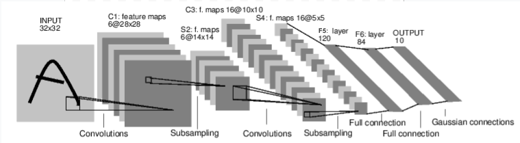

Transformer

import torch
import torch.nn as nn

class TransformerClassifier(nn.Module):
    def __init__(self, vocab_size, d_model=512, nhead=8, num_layers=2, num_classes=2):
        super(TransformerClassifier, self).__init__()
        self.embedding = nn.Embedding(vocab_size, d_model)
        self.pos_encoder = nn.Parameter(torch.randn(1, 100, d_model))  # Max seq len = 100
        encoder_layer = nn.TransformerEncoderLayer(d_model=d_model, nhead=nhead, batch_first=True)
        self.transformer_encoder = nn.TransformerEncoder(encoder_layer, num_layers=num_layers)
        self.fc = nn.Linear(d_model, num_classes)

    def forward(self, x):
        # x: [batch_size, seq_len] (token indices)
        x = self.embedding(x) + self.pos_encoder[:, :x.size(1), :]  # Add positional encoding
        x = self.transformer_encoder(x)  # [batch_size, seq_len, d_model]
        x = x.mean(dim=1)  # Pool over sequence length
        logits = self.fc(x)  # [batch_size, num_classes]
        return logits

# Example usage
device = torch.device("cuda" if torch.cuda.is_available() else "cpu")
model = TransformerClassifier(vocab_size=10000).to(device)
print(model)

AlexNet

import torch
import torch.nn as nn

class AlexNet(nn.Module):
    def __init__(self, num_classes=1000):
        super(AlexNet, self).__init__()
        self.features = nn.Sequential(
            nn.Conv2d(3, 64, kernel_size=11, stride=4, padding=2),  # 3x224x224 -> 64x55x55
            nn.ReLU(inplace=True),
            nn.MaxPool2d(kernel_size=3, stride=2),  # 64x55x55 -> 64x27x27
            nn.Conv2d(64, 192, kernel_size=5, padding=2),  # 64x27x27 -> 192x27x27
            nn.ReLU(inplace=True),
            nn.MaxPool2d(kernel_size=3, stride=2),  # 192x27x27 -> 192x13x13
            nn.Conv2d(192, 384, kernel_size=3, padding=1),  # 192x13x13 -> 384x13x13
            nn.ReLU(inplace=True),
            nn.Conv2d(384, 256, kernel_size=3, padding=1),  # 384x13x13 -> 256x13x13
            nn.ReLU(inplace=True),
            nn.Conv2d(256, 256, kernel_size=3, padding=1),  # 256x13x13 -> 256x13x13
            nn.ReLU(inplace=True),
            nn.MaxPool2d(kernel_size=3, stride=2),  # 256x13x13 -> 256x6x6
        )
        self.classifier = nn.Sequential(
            nn.Flatten(),
            nn.Dropout(p=0.5),
            nn.Linear(256 * 6 * 6, 4096),
            nn.ReLU(inplace=True),
            nn.Dropout(p=0.5),
            nn.Linear(4096, 4096),
            nn.ReLU(inplace=True),
            nn.Linear(4096, num_classes),
        )

    def forward(self, x):
        x = self.features(x)
        x = self.classifier(x)
        return x

# Example usage
device = torch.device("cuda" if torch.cuda.is_available() else "cpu")
model = AlexNet(num_classes=1000).to(device)
print(model)

ResNet18

ResNet18之所以叫“18”，是因为它的网络架构包含18个带权重的层（即卷积层和全连接层）。

import torch
import torch.nn as nn
import torch.nn.functionl as F

#定义残差块ResBlock
class ResBlock(nn.Module):
    def __init__(self, inchannel, outchannel, stride=1):
        super(ResBlock, self).__init__()
        #这里定义了残差块内连续的2个卷积层
        self.left = nn.Sequential(
            nn.Conv2d(inchannel, outchannel, kernel_size=3, stride=stride, padding=1, bias=False),
            nn.BatchNorm2d(outchannel),
            nn.ReLU(inplace=True),
            nn.Conv2d(outchannel, outchannel, kernel_size=3, stride=1, padding=1, bias=False),
            nn.BatchNorm2d(outchannel)
        )
        self.shortcut = nn.Sequential()
        if stride != 1 or inchannel != outchannel:
            #shortcut，这里为了跟2个卷积层的结果结构一致，要做处理
            self.shortcut = nn.Sequential(
                nn.Conv2d(inchannel, outchannel, kernel_size=1, stride=stride, bias=False),
                nn.BatchNorm2d(outchannel)
            )

    def forward(self, x):
        out = self.left(x)
        #将2个卷积层的输出跟处理过的x相加，实现ResNet的基本结构
        out = out + self.shortcut(x)
        out = F.relu(out)

        return out

class ResNet(nn.Module):
    def __init__(self, ResBlock, num_classes=10):
        super(ResNet, self).__init__()
        self.inchannel = 64
        self.conv1 = nn.Sequential(
            nn.Conv2d(3, 64, kernel_size=3, stride=1, padding=1, bias=False),
            nn.BatchNorm2d(64),
            nn.ReLU()
        )
        self.layer1 = self.make_layer(ResBlock, 64, 2, stride=1)
        self.layer2 = self.make_layer(ResBlock, 128, 2, stride=2)
        self.layer3 = self.make_layer(ResBlock, 256, 2, stride=2)        
        self.layer4 = self.make_layer(ResBlock, 512, 2, stride=2)        
        self.fc = nn.Linear(512, num_classes)
    #这个函数主要是用来，重复同一个残差块    
    def make_layer(self, block, channels, num_blocks, stride):
        strides = [stride] + [1] * (num_blocks - 1)
        layers = []
        for stride in strides:
            layers.append(block(self.inchannel, channels, stride))
            self.inchannel = channels
        return nn.Sequential(*layers)

    def forward(self, x):
        #在这里，整个ResNet18的结构就很清晰了
        out = self.conv1(x)
        out = self.layer1(out)
        out = self.layer2(out)
        out = self.layer3(out)
        out = self.layer4(out)
        out = F.avg_pool2d(out, 4)
        out = out.view(out.size(0), -1)
        out = self.fc(out)
        return out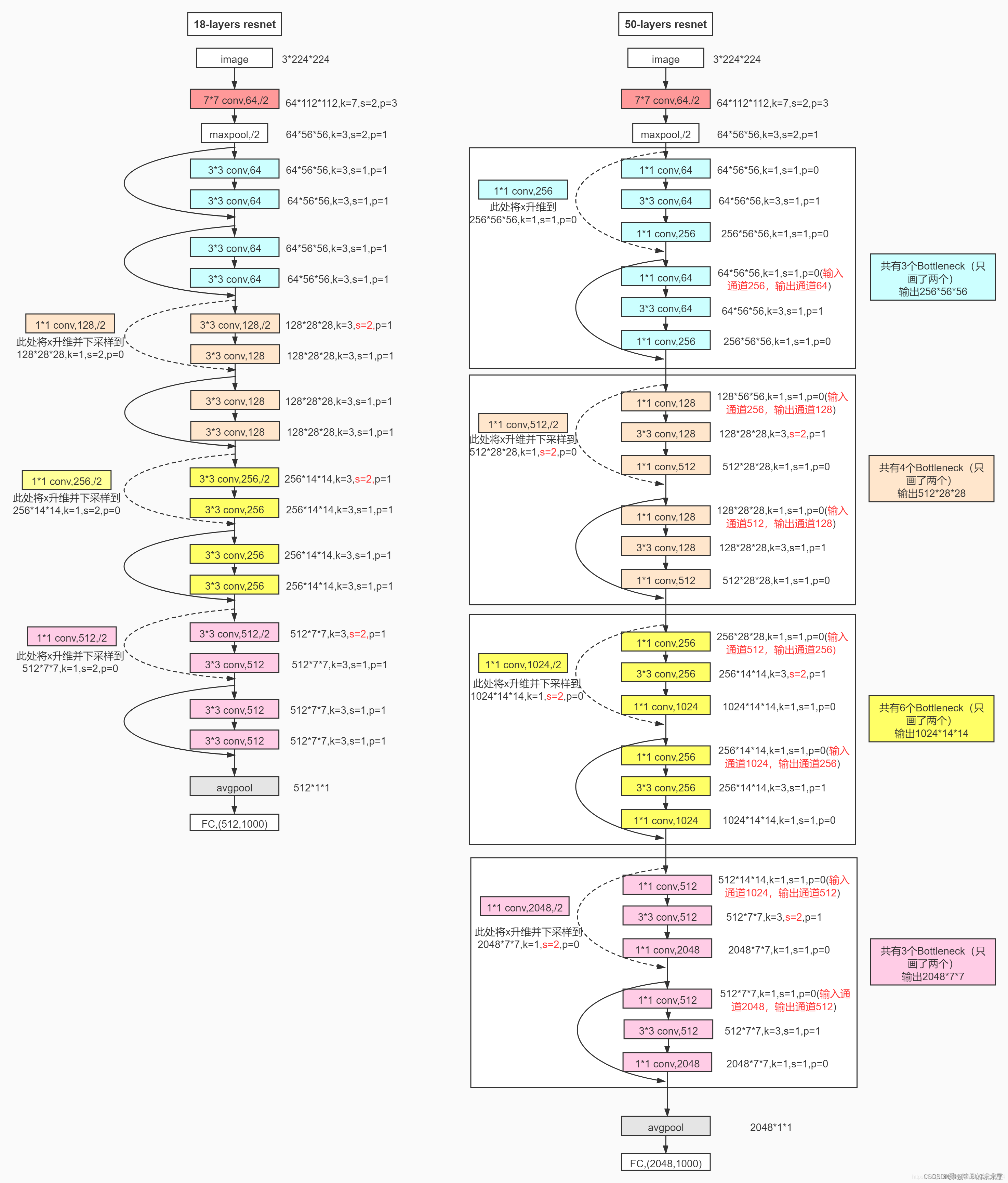

UNet

import ddpm 
from PIL import Image
from torchvision import transforms
import torch
from torch import nn
import matplotlib.pyplot as plt
import numpy as np

image = Image.open("giraffe.jpg")

image_size = 128
transform = transforms.Compose([
    transforms.Resize(image_size),
    transforms.CenterCrop(image_size),
    transforms.PILToTensor(),
    transforms.ConvertImageDtype(torch.float),
    transforms.Normalize(mean=[0.5, 0.5, 0.5], std=[0.5, 0.5, 0.5]),
])

x_start = transform(image).unsqueeze(0)

diffusion_linear = ddpm.Diffusion(noise_steps=500)
diffusion_cosine = ddpm.Diffusion(noise_steps=500,beta_schedule='cosine')

plt.figure(figsize=(16, 8))
for idx, t in enumerate([0, 50, 100, 200, 499]): 
    x_noisy,_ = diffusion_linear.q_sample(x_start, t=torch.tensor([t])) # 使用q_sample去生成x_t
    x_noisy2,_ = diffusion_cosine.q_sample(x_start,t=torch.tensor([t])) # [1,3,128,128]
    noisy_image = (x_noisy.squeeze().permute(1, 2, 0) + 1) * 127.5  # 我们的x_t被裁剪到（-1，1）,所以+1后乘以127.5
    noisy_img2 = (x_noisy2.squeeze().permute(1,2,0)+1)*127.5 # # [128,128,3] -> (0,2) 
    noisy_image = noisy_image.numpy().astype(np.uint8)
    noisy_img2 = noisy_img2.numpy().astype(np.uint8)
    plt.subplot(2, 5, 1 + idx)
    plt.imshow(noisy_image)
    plt.axis("off")
    plt.title(f"t={t}")
    plt.subplot(2, 5, 6+idx)
    plt.imshow(noisy_img2)
    plt.axis('off')
plt.figtext(0.5, 0.95, 'Linear Beta Schedule', ha='center', fontsize=16)  # 在第一行上方添加大标题
plt.figtext(0.5, 0.48, 'Cosine Beta Schedule', ha='center', fontsize=16)  # 在第二行上方添加大标题
plt.savefig('temp_img/add_noise_process.png')

class SelfAttention(nn.Module):
    def __init__(self,channels):
        super().__init__()
        self.channels = channels
        self.mha = nn.MultiheadAttention(channels, 4, batch_first=True)
        self.ln = nn.LayerNorm([channels])
        self.ff = nn.Sequential(
            nn.LayerNorm([channels]),
            nn.Linear(channels,channels),
            nn.GELU(),
            nn.Linear(channels,channels)
            )

    def forward(self,x):
        B,C,H,W = x.shape
        x = x.reshape(-1,self.channels,H*W).swapaxes(1,2)
        x_ln = self.ln(x)
        attention_value = self.mha(x_ln)
        attention_value = attention_value + x
        attention_value = self.ff(attention_value)+ attention_value
        return attention_value.swapaxes(1,2).view(-1,self.channels,H,W)

class DoubleConv(nn.Module):
    def __init__(self,in_c,out_c,mid_c=None,residual=False):
        super().__init__()
        self.residual = residual
        if mid_c is None:
            mid_c = out_c
        self.double_conv = nn.Sequential(
            nn.Conv2d(in_c,mid_c,kernel_size=3,padding=1),
            nn.GroupNorm(1,mid_c),
            nn.GELU(),
            nn.Conv2d(mid_c,out_c,kernel_size=3,padding=1),
            nn.GroupNorm(1,mid_c)
            )
        if in_c != out_c:
            self.shortcut = nn.Conv2d(in_c,out_c,kernel_size=1)
        else:
            self.shortcut = nn.Identity()

    def forward(self,x):
        if self.residual:
            return F.gelu(self.shortcut(x)+self.double_conv(x))
        else:
            return F.gelu(self.double_conv(x))

class Down(nn.Module):
    def __init__(self,in_c,out_c,emb_dim=256):
        self.maxpool_conv = nn.Sequential(
            nn.MaxPool2d(2) # kernel_size=2, stride default equal to k
            DoubleConv(in_c,out_c,residual=True),
            DoubleConv(out_c,out_c)
            )
        self.emb_layer = nn.Sequential(
            nn.SiLU(),
            nn.Linear(emb_dim,out_c)
            )

    def forward(self,x,t):
        x = self.maxpool_conv(x)
        emb = self.emb_layer(t)[:,:,None,None].repeat(1,1,x.shape[-2],x.shape[-1])
        # 扩维后，在最后两维重复h和w次，此时和x的尺寸相同
        return x+emb

class Up(nn.Module):
    def __init__(self,in_c,out_c,emb_dim=256):
        self.up =  nn.UpSample(scale_factor=2,mode='bilinear', align_corner=True)
        self.conv = nn.Sequential(
            nn.Conv2d(in_c,in_c,residual=True),
            nn.Conv2d(in_c,out_c)
            )
        self.emb_layer = nn.Sequential(
            nn.SiLU(),
            nn.Linear(emb_dim,out_c)
            )

    def forward(self,x,skip_x, t):
        x = self.up(x)
        x = torch.cat([x,skip_x],dim=1)
        x = self.conv(x)
        emb = self.emb_layer(t)[:,:,None,None].repeat(1,1,x.shape[-2],x.shape[-1])
        return x + emb

class UNet(nn.Module):
    def __init__(self,in_c, out_c, time_dim=256, device='cuda'):
        super().__init__()
        self.device = device
        self.time_dim = time_dim
        self.inc = DoubleConv(c_in, 64)
        self.down1 = Down(64, 128)
        self.sa1 = SelfAttention(128)
        self.down2 = Down(128, 256)
        self.sa2 = SelfAttention(256)
        self.down3 = Down(256, 512)
        self.sa3 = SelfAttention(512)

        self.bot1 = DoubleConv(512, 512)
        self.bot2 = DoubleConv(512, 512)
        self.bot3 = DoubleConv(512, 256)

        self.up1 = Up(512, 128)
        self.sa4 = SelfAttention(128)
        self.up2 = Up(256, 64)
        self.sa5 = SelfAttention(64)
        self.up3 = Up(128, 64)
        self.sa6 = SelfAttention(64)
        self.outc = nn.Conv2d(64, c_out, kernel_size=1)

    def pos_encoding(self,t,channels):
        freq = 1.0/(10000**torch.arange(0,channels,2,device=self.device).float()/channels)
        args = t[:,None].float()*freq[None]
        embedding = torch.cat([torch.sin(args), torch.cos(args)],dim=-1)
        if channels % 2 != 0:
            embedding = torch.cat([embedding,torch.zeros_like(embedding[:,:1])],dim=-1)
        return embeddig

    def forward(self,x,t):
        t = self.pos_encoding(t,self.time_dim)
        x1 = self.inc(x)
        x2 = self.down1(x1, t)
        x2 = self.sa1(x2)
        x3 = self.down2(x2, t)
        x3 = self.sa2(x3)
        x4 = self.down3(x3, t)
        x4 = self.sa3(x4)

        x4 = self.bot1(x4)
        x4 = self.bot2(x4)
        x4 = self.bot3(x4)

        x = self.up1(x4, x3, t)
        x = self.sa4(x)
        x = self.up2(x, x2, t)
        x = self.sa5(x)
        x = self.up3(x, x1, t)
        x = self.sa6(x)
        output = self.outc(x)
        return output

    def linear_beta_schedule(self):
        scale = 1000/self.noise_steps
        beta_start = self.beta_start*scale
        beta_end = self.beta_end*scale
        return torch.linspace(beta_start, beta_end, self.noise_steps)

    def cosine_beta_schedule(self,s=0.008):
        """
        as proposed in Improved ddpm paper;
        """
        steps = self.noise_steps + 1
        x = torch.linspace(0, self.noise_steps, steps, dtype=torch.float64) # 从0到self.noise_steps
        alphas_cumprod = torch.cos(((x / self.noise_steps) + s) / (1 + s) * math.pi * 0.5) ** 2
        alphas_cumprod = alphas_cumprod / alphas_cumprod[0]
        betas = 1 - (alphas_cumprod[1:] / alphas_cumprod[:-1]) # alpha_cumprod包含了noise_steps+1个值，则alpha_t是第一个到最后一个；alpha_{t-1}是第0个到倒数第二个（第0个为0）
        return torch.clip(betas, 0, 0.999) # 不大于0.999

class Diffusion:
    def __init__(self, noise_steps=1000, beta_start=1e-4, beta_end=0.02, img_size=256, beta_schedule='linear',device="cuda"):
        self.noise_steps = noise_steps
        self.beta_start = beta_start
        self.beta_end = beta_end
        self.img_size = img_size
        self.device = device
        if beta_schedule == 'linear':
            self.beta = self.linear_beta_schedule().to(device)
        elif beta_schedule == 'cosine':
            self.beta = self.cosine_beta_schedule().to(device)
        else:
            raise ValueError(f'Unknown beta schedule {beta_schedule}')

        # all parameters
        self.alpha = 1. - self.beta 
        self.alpha_hat = torch.cumprod(self.alpha, dim=0) 
        self.alpha_hat_prev = F.pad(self.alpha_hat[:-1],(1,0),value=1.)
        self.sqrt_alpha_hat = torch.sqrt(self.alpha_hat)
        self.sqrt_one_minus_alpha_hat = torch.sqrt(1.-self.alpha_hat)
        self.sqrt_recip_alpha_hat = torch.sqrt(1./self.alpha_hat) # 用于估计x_0，估计x_0后用于计算p(x_{t-1}|x_t) 均值
        self.sqrt_recip_minus_alpha_hat = torch.sqrt(1./self.alpha_hat-1) 
        self.posterior_variance = (self.beta*(1.-self.alpha_hat_prev)/(1.-self.alpha_hat)) # 用于计算p(x_{t-1}|x_t)的方差
        self.posterior_mean_coef1 = (self.beta * torch.sqrt(self.alpha_hat_prev) / (1.0 - self.alphas_hat)) # 用于计算p(x_{t-1}|x_t)的均值
        self.posterior_mean_coef2 = ((1.0 - self.alphas_hat_prev)* torch.sqrt(self.alphas)/ (1.0 - self.alphas_hat))

    def _extract(self,arr,t,x_shape):
        # 根据timestep t从arr中提取对应元素并变形为x_shape
        bs = x_shape[0]
        out = arr.to(t.device).gather(0,t).float()
        out = out.reshape(bs,*((1,)*(len(x_shape)-1))) # reshape为(bs,1,1,1)
        return out

    def q_sample(self, x, t, noise=None):
        # q(x_t|x_0)
        if noise is None:
            Ɛ = torch.randn_like(x)
        sqrt_alpha_hat = self._extract(self.sqrt_alpha_hat,t,x.shape)
        sqrt_one_minus_alpha_hat = self._extract(self.sqrt_one_minus_alpha_hat,t,x.shape)
        return sqrt_alpha_hat * x + sqrt_one_minus_alpha_hat * Ɛ, Ɛ

    def q_posterior_mean_variance(self,x,x_t,t):
        # calculate mean and variance of q(x_{t-1}|x_t,x_0), we send parameters x0 and x_t into this function
        # in fact we use this function to predict p(x_{t-1}|x_t)'s mean and variance by sending x_t, \hat x_0, t
        posterior_mean =  (
            self._extract(self.posterior_mean_coef1,t,x.shape) * x 
            + self._extract(self.posterior_mean_coef2,t,x.shape) * x_t
        )
        posterior_variance = (self.posterior_variance,t,x.shape)
        return posterior_mean, posterior_variance

    def estimate_x0_from_noise(self,x_t,t,noise):
        # \hat x_0
        return (self._extract(self.sqrt_recip_alpha_hat,t,x_t.shape)*x_t + self._extract(self.sqrt_recip_minus_alpha_hat,t,x_t.shape)*noise)

    def p_mean_variance(self,model,x_t,t,clip_denoised=True):
        pred_noise = model(x_t,t)
        x_recon = self.estimate_x0_from_noise(x_t,t,pred_noise)
        if clip_denoised:
            x_recon = torch.clamp(x_recon,min=-1.,max=1.)
        p_mean,p_var = self.q_posterior_mean_variance(x_recon,x_t,t)
        return p_mean,p_var

    def p_sample(self, model, x_t, t, clip_denoised=True):
        logging.info(f"Sampling {n} new images....")
        model.eval()
        with torch.no_grad():
            p_mean,p_var = self.p_mean_variance(model,x_t,t,clip_denoised=clip_denoised)
            noise = torch.randn_like(x_t)
            nonzero_mask = ((t!=0).float().view(-1,*([1]*len(x_t.shape)-1))) # 当t!=0时为1，否则为0
            pred_img = p_mean + nonzero_mask*(torch.sqrt(p_var))*noise
        return pred_img

    def p_sample_loop(self,model,shape):
        model.eval()
        with torch.no_grad():
            bs = shape[0]
            device = next(model.parameters()).to(device)
            img = torch.randn(shape,device=device)
            imgs = []
            for i in tqdm(reversed(range(0,self.noise_steps)),desc='sampling loop time step',total=self.noise_steps):
                img = self.p_sample(model,img,torch.full((bs,),i,device=device,dtype=torch.long)) # 从T到0
                imgs.append(img)
        return imgs

    @torch.no_grad()
    def sample(self,model,img_size,bs=8,channels=3):
        return self.p_sample_loop(model,(bs,channels,img_size,img_size))

def train(args):
    setup_logging(args.run_name)
    device = args.device
    dataloader = get_data(args)
    model = UNet().to(device)
    optimizer = optim.AdamW(model.parameters(), lr=args.lr)
    mse = nn.MSELoss()
    diffusion = Diffusion(img_size=args.image_size, device=device)
    logger = SummaryWriter(os.path.join("runs", args.run_name))
    l = len(dataloader)

    for epoch in range(args.epochs):
        logging.info(f"Starting epoch {epoch}:")
        pbar = tqdm(dataloader)
        for i, (images, _) in enumerate(pbar):
            images = images.to(device)
            t = diffusion.sample_timesteps(images.shape[0]).to(device)
            x_t, noise = diffusion.q_sample(images, t)
            predicted_noise = model(x_t, t)
            loss = mse(noise, predicted_noise)

            optimizer.zero_grad()
            loss.backward()
            optimizer.step()

            pbar.set_postfix(MSE=loss.item())
            logger.add_scalar("MSE", loss.item(), global_step=epoch * l + i)

        sampled_images = diffusion.sample(model, n=images.shape[0])
        save_images(sampled_images, os.path.join("results", args.run_name, f"{epoch}.jpg"))
        torch.save(model.state_dict(), os.path.join("models", args.run_name, f"ckpt.pt"))

def launch():
    import argparse
    parser = argparse.ArgumentParser()
    args = parser.parse_args()
    args.run_name = "DDPM_Uncondtional"
    args.epochs = 500
    args.batch_size = 12
    args.image_size = 64
    args.dataset_path = r"C:\Users\dome\datasets\landscape_img_folder"
    args.device = "cuda"
    args.lr = 3e-4
    train(args)

if __name__ == '__main__':
    launch()

HaibinLai/Bike-sharing-or-Uber at 9afceaf7e1acf6acc23e82ea5d73877448548878

RNN

import torch
import torch.nn as nn
import random
from logging import getLogger
from libcity.model import loss
from libcity.model.abstract_traffic_state_model import AbstractTrafficStateModel

class RNN(AbstractTrafficStateModel):
    def __init__(self, config, data_feature):
        super().__init__(config, data_feature)
        self._scaler = self.data_feature.get('scaler')
        self.num_nodes = self.data_feature.get('num_nodes', 1)
        self.feature_dim = self.data_feature.get('feature_dim', 1)
        self.output_dim = self.data_feature.get('output_dim', 1)

        self.input_window = config.get('input_window', 1)
        self.output_window = config.get('output_window', 1)
        self.device = config.get('device', torch.device('cpu'))
        self._logger = getLogger()
        self._scaler = self.data_feature.get('scaler')

        self.rnn_type = config.get('rnn_type', 'RNN')
        self.hidden_size = config.get('hidden_size', 64)
        self.num_layers = config.get('num_layers', 1)
        self.dropout = config.get('dropout', 0)
        self.bidirectional = config.get('bidirectional', False)
        self.teacher_forcing_ratio = config.get('teacher_forcing_ratio', 0)
        if self.bidirectional:
            self.num_directions = 2
        else:
            self.num_directions = 1
        self.input_size = self.num_nodes * self.feature_dim

        self._logger.info('You select rnn_type {} in RNN!'.format(self.rnn_type))
        if self.rnn_type.upper() == 'GRU':
            self.rnn = nn.GRU(input_size=self.input_size, hidden_size=self.hidden_size,
                              num_layers=self.num_layers, dropout=self.dropout,
                              bidirectional=self.bidirectional)
        elif self.rnn_type.upper() == 'LSTM':
            self.rnn = nn.LSTM(input_size=self.input_size, hidden_size=self.hidden_size,
                               num_layers=self.num_layers, dropout=self.dropout,
                               bidirectional=self.bidirectional)
        elif self.rnn_type.upper() == 'RNN':
            self.rnn = nn.RNN(input_size=self.input_size, hidden_size=self.hidden_size,
                              num_layers=self.num_layers, dropout=self.dropout,
                              bidirectional=self.bidirectional)
        else:
            raise ValueError('Unknown RNN type: {}'.format(self.rnn_type))
        self.fc = nn.Linear(self.hidden_size * self.num_directions, self.num_nodes * self.output_dim)

    def forward(self, batch):
        src = batch['X'].clone()  # [batch_size, input_window, num_nodes, feature_dim]
        target = batch['y']  # [batch_size, output_window, num_nodes, feature_dim]
        src = src.permute(1, 0, 2, 3)  # [input_window, batch_size, num_nodes, feature_dim]
        target = target.permute(1, 0, 2, 3)  # [output_window, batch_size, num_nodes, output_dim]

        batch_size = src.shape[1]
        src = src.reshape(self.input_window, batch_size, self.num_nodes * self.feature_dim)
        # src = [self.input_window, batch_size, self.num_nodes * self.feature_dim]
        outputs = []
        for i in range(self.output_window):
            # src: [input_window, batch_size, num_nodes * feature_dim]
            out, _ = self.rnn(src)
            # out: [input_window, batch_size, hidden_size * num_directions]
            out = self.fc(out[-1])
            # out: [batch_size, num_nodes * output_dim]
            out = out.reshape(batch_size, self.num_nodes, self.output_dim)
            # out: [batch_size, num_nodes, output_dim]
            outputs.append(out.clone())
            if self.output_dim < self.feature_dim:  # output_dim可能小于feature_dim
                out = torch.cat([out, target[i, :, :, self.output_dim:]], dim=-1)
            # out: [batch_size, num_nodes, feature_dim]
            if self.training and random.random() < self.teacher_forcing_ratio:
                src = torch.cat((src[1:, :, :], target[i].reshape(
                    batch_size, self.num_nodes * self.feature_dim).unsqueeze(0)), dim=0)
            else:
                src = torch.cat((src[1:, :, :], out.reshape(
                    batch_size, self.num_nodes * self.feature_dim).unsqueeze(0)), dim=0)
        outputs = torch.stack(outputs)
        # outputs = [output_window, batch_size, num_nodes, output_dim]
        return outputs.permute(1, 0, 2, 3)

    def calculate_loss(self, batch):
        y_true = batch['y']
        y_predicted = self.predict(batch)
        y_true = self._scaler.inverse_transform(y_true[..., :self.output_dim])
        y_predicted = self._scaler.inverse_transform(y_predicted[..., :self.output_dim])
        return loss.masked_mae_torch(y_predicted, y_true, 0)

    def predict(self, batch):
        return self.forward(batch)

ConvGCN

from libcity.model import loss
from libcity.model.abstract_traffic_state_model import AbstractTrafficStateModel
import torch.nn.functional as F
import math
import torch
import torch.nn as nn
from torch.nn.parameter import Parameter
from torch.nn.modules.module import Module

"""
输入流入和流出的2维数据
"""

class GraphConvolution(Module):
    def __init__(self, in_features, out_features, device, bias=True):
        super(GraphConvolution, self).__init__()
        self.in_features = in_features
        self.out_features = out_features
        self.weight = Parameter(torch.FloatTensor(in_features, out_features).to(device))  # FloatTensor建立tensor
        if bias:
            self.bias = Parameter(torch.FloatTensor(1, out_features, 1, 1)).to(device)
        else:
            self.register_parameter('bias', None)
        self.reset_parameters()

    # 初始化权重
    def reset_parameters(self):
        stdv = 1. / math.sqrt(self.weight.size(0))
        self.weight.data.uniform_(-stdv, stdv)
        if self.bias is not None:
            self.bias.data.uniform_(-stdv, stdv)

    def forward(self, input, adjT):
        # print('input.shape:', input.shape)
        # print('self.weight.shape:', self.weight.shape)
        support = torch.einsum("ijkl, jm->imkl", [input, self.weight])
        # print('support.shape:', support.shape)
        # print('adjT.shape:', adjT.shape)
        output = torch.einsum("ak, ijkl->ijal", [adjT, support])
        # print('output.shape:', output.shape)
        # print('self.bias.shape:', self.bias.shape)
        if self.bias is not None:
            return output + self.bias
        else:
            return output

class GCN(nn.Module):
    def __init__(self, input_size, hidden_size, output_size, device):
        super(GCN, self).__init__()

        self.gc1 = GraphConvolution(input_size, hidden_size, device)
        self.gc2 = GraphConvolution(hidden_size, output_size, device)

    def forward(self, x, adj):
        x = F.relu(self.gc1(x, adj))
        x = self.gc2(x, adj)
        return x

class CONVGCN(AbstractTrafficStateModel):
    def __init__(self, config, data_feature):
        super().__init__(config, data_feature)
        self.device = config.get('device', torch.device('cpu'))
        self._scaler = self.data_feature.get('scaler')
        self.adj_mx = torch.tensor(self.data_feature.get('adj_mx'), device=self.device)
        self.num_nodes = self.data_feature.get('num_nodes', 1)
        for i in range(self.num_nodes):
            self.adj_mx[i, i] = 1
        self.feature_dim = self.data_feature.get('feature_dim', 1)  # 输入维度
        self.output_dim = self.data_feature.get('output_dim', 1)  # 输出维度
        # self._logger = getLogger()
        self.conv_depth = config.get('conv_depth', 5)
        self.conv_height = config.get('conv_height', 3)
        self.hidden_size = config.get('hidden_size', 16)
        self.time_lag = config.get('time_lag', 1)
        self.output_window = config.get('output_window', 1)

        self.gc = GCN(
            (self.time_lag-1) * 3,
            self.hidden_size,
            self.conv_depth * self.conv_height,
            self.device
        )
        self.Conv = nn.Conv3d(
            in_channels=self.num_nodes,
            out_channels=self.num_nodes,
            kernel_size=3,
            stride=(1, 1, 1),
            padding=(1, 1, 1)
        )
        self.relu = nn.ReLU()
        self.fc = nn.Linear(
            self.num_nodes * self.conv_depth * self.conv_height * self.feature_dim,
            self.num_nodes * self.output_window * self.output_dim
        )

    def forward(self, batch):

        x = batch['X']
        out = self.gc(x, self.adj_mx)
        # print('gc_output:', out.shape)
        out = torch.reshape(
            out,
            (-1, self.num_nodes, self.conv_depth, self.conv_height, self.feature_dim)
        )
        # print('conv_in:', out.shape)
        out = self.relu(self.Conv(out))
        # print('conv_out:', out.shape)

        out = out.view(-1, self.num_nodes * self.conv_depth * self.conv_height * self.feature_dim)
        out = self.fc(out)
        out = torch.reshape(out, [-1, self.output_window, self.num_nodes, self.output_dim])
        return out

    def predict(self, batch):
        return self.forward(batch)

    def calculate_loss(self, batch):
        y_true = batch['y']
        y_predicted = self.predict(batch)
        # print('size of y_true:', y_true.shape)
        # print('size of y_predict:', y_predicted.shape)
        y_true = self._scaler.inverse_transform(y_true[..., :self.output_dim])
        y_predicted = self._scaler.inverse_transform(y_predicted[..., :self.output_dim])
        return loss.masked_mse_torch(y_predicted, y_true, 0)

自动微分

Automatic Differentiation with torch.autograd — PyTorch Tutorials 2.7.0+cu126 documentation
A Gentle Introduction to torch.autograd — PyTorch Tutorials 2.7.0+cu126 documentation

import torch

x = torch.ones(5)  # input tensor
y = torch.zeros(3)  # expected output
w = torch.randn(5, 3, requires_grad=True)
b = torch.randn(3, requires_grad=True)
z = torch.matmul(x, w)+b
loss = torch.nn.functional.binary_cross_entropy_with_logits(z, y)

Conceptually, autograd keeps a record of data (tensors) & all executed operations (along with the resulting new tensors) in a directed acyclic graph (DAG) consisting of Function objects. In this DAG, leaves are the input tensors, roots are the output tensors. By tracing this graph from roots to leaves, you can automatically compute the gradients using the chain rule.
In a forward pass, autograd does two things simultaneously:

• run the requested operation to compute a resulting tensor, and
• maintain the operation’s gradient function in the DAG.

The backward pass kicks off when .backward() is called on the DAG root. autograd then:

• computes the gradients from each .grad_fn,
• accumulates them in the respective tensor’s .grad attribute, and
• using the chain rule, propagates all the way to the leaf tensors.

Below is a visual representation of the DAG in our example. In the graph, the arrows are in the direction of the forward pass. The nodes represent the backward functions of each operation in the forward pass. The leaf nodes in blue represent our leaf tensors a and b.

By default, all tensors with requires_grad=True are tracking their computational history and support gradient computation. However, there are some cases when we do not need to do that, for example, when we have trained the model and just want to apply it to some input data, i.e. we only want to do forward computations through the network. We can stop tracking computations by surrounding our computation code with torch.no_grad() block:

z = torch.matmul(x, w)+b
print(z.requires_grad) # True

with torch.no_grad():
    z = torch.matmul(x, w)+b
print(z.requires_grad) # False

Autograd mechanics — PyTorch 2.7 documentation

import torch

# 创建张量，启用梯度追踪
x = torch.tensor(2.0, requires_grad=True)
y = x**2 + 3*x + 1  # 前向计算

# 反向传播
y.backward()

# 梯度存储在 x.grad 中
print(x.grad)  # 输出：dy/dx = 2x + 3 = 2*2 + 3 = 7

训练

To train a model, we need a loss function and an optimizer.

loss_fn = nn.CrossEntropyLoss()
optimizer = torch.optim.SGD(model.parameters(), lr=1e-3)

In a single training loop, the model makes predictions on the training dataset (fed to it in batches), and backpropagates the prediction error to adjust the model’s parameters.

# 查看size
batch_size = 64

def train(dataloader, model, loss_fn, optimizer):
    size = len(dataloader.dataset)
    model.train() # Set the model to training mode
    for batch, (X, y) in enumerate(dataloader):
        X, y = X.to(device), y.to(device) # put data into device

        # Compute prediction error
        pred = model(X)
        loss = loss_fn(pred, y) # the loss func we init

        # Backpropagation
        loss.backward()
        optimizer.step() # how much we should step
        optimizer.zero_grad()

        if batch % 100 == 0:
            loss, current = loss.item(), (batch + 1) * len(X)
            print(f"loss: {loss:>7f}  [{current:>5d}/{size:>5d}]")

测试Test & Eval

def test(dataloader, model, loss_fn):
    size = len(dataloader.dataset)
    num_batches = len(dataloader)
    model.eval()
    test_loss, correct = 0, 0
    with torch.no_grad():
        for X, y in dataloader:
            X, y = X.to(device), y.to(device)
            pred = model(X)
            test_loss += loss_fn(pred, y).item()
            correct += (pred.argmax(1) == y).type(torch.float).sum().item()
    test_loss /= num_batches
    correct /= size
    print(f"Test Error: \n Accuracy: {(100*correct):>0.1f}%, Avg loss: {test_loss:>8f} \n")

The training process is conducted over several iterations (epochs). During each epoch, the model learns parameters to make better predictions. We print the model’s accuracy and loss at each epoch; we’d like to see the accuracy increase and the loss decrease with every epoch.

epochs = 5
for t in range(epochs):
    print(f"Epoch {t+1}\n-------------------------------")
    train(train_dataloader, model, loss_fn, optimizer)
    test(test_dataloader, model, loss_fn)
print("Done!")

def train_loop(dataloader, model, loss_fn, optimizer):
    size = len(dataloader.dataset)
    # Set the model to training mode - important for batch normalization and dropout layers
    # Unnecessary in this situation but added for best practices
    model.train()
    for batch, (X, y) in enumerate(dataloader):
        # Compute prediction and loss
        pred = model(X)
        loss = loss_fn(pred, y)

        # Backpropagation
        loss.backward()
        optimizer.step()
        optimizer.zero_grad()

        if batch % 100 == 0:
            loss, current = loss.item(), batch * batch_size + len(X)
            print(f"loss: {loss:>7f}  [{current:>5d}/{size:>5d}]")

def test_loop(dataloader, model, loss_fn):
    # Set the model to evaluation mode - important for batch normalization and dropout layers
    # Unnecessary in this situation but added for best practices
    model.eval()
    size = len(dataloader.dataset)
    num_batches = len(dataloader)
    test_loss, correct = 0, 0

    # Evaluating the model with torch.no_grad() ensures that no gradients are computed during test mode
    # also serves to reduce unnecessary gradient computations and memory usage for tensors with requires_grad=True
    with torch.no_grad():
        for X, y in dataloader:
            pred = model(X)
            test_loss += loss_fn(pred, y).item()
            correct += (pred.argmax(1) == y).type(torch.float).sum().item()

    test_loss /= num_batches
    correct /= size
    print(f"Test Error: \n Accuracy: {(100*correct):>0.1f}%, Avg loss: {test_loss:>8f} \n")

不同的fig

保存模型 & 加载模型

Save and Load the Model — PyTorch Tutorials 2.7.0+cu126 documentation

torch.save(model.state_dict(), "model.pth")
print("Saved PyTorch Model State to model.pth")

model = NeuralNetwork().to(device)
model.load_state_dict(torch.load("model.pth", weights_only=True))

This model can now be used to make predictions.

classes = [
    "T-shirt/top",
    "Trouser",
    "Pullover",
    "Dress",
    "Coat",
    "Sandal",
    "Shirt",
    "Sneaker",
    "Bag",
    "Ankle boot",
]

model.eval()
x, y = test_data[0][0], test_data[0][1]
with torch.no_grad():
    x = x.to(device)
    pred = model(x)
    predicted, actual = classes[pred[0].argmax(0)], classes[y]
    print(f'Predicted: "{predicted}", Actual: "{actual}"')

如何用Profiler profile并且优化

Profiling your PyTorch Module — PyTorch Tutorials 2.7.0+cu126 documentation
Automatic differentiation package - torch.autograd — PyTorch 2.7 documentation

A guide on good usage of non_blocking and pin_memory() in PyTorch — PyTorch Tutorials 2.7.0+cu126 documentation

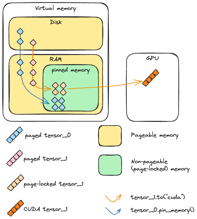
Optimizing the transfer of tensors from the CPU to the GPU can be achieved through asynchronous transfers and memory pinning. However, there are important considerations:

• Using tensor.pin_memory().to(device, non_blocking=True) can be up to twice as slow as a straightforward tensor.to(device).
• Generally, tensor.to(device, non_blocking=True) is an effective choice for enhancing transfer speed.
• While cpu_tensor.to("cuda", non_blocking=True).mean() executes correctly, attempting cuda_tensor.to("cpu", non_blocking=True).mean() will result in erroneous outputs.

Holistic Trace Analysis

Introduction to Holistic Trace Analysis — PyTorch Tutorials 2.7.0+cu126 documentation

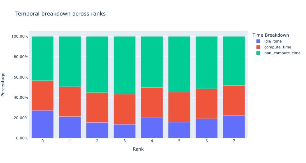
Kernel Duration DistributionKDD

The second dataframe returned by get_gpu_kernel_breakdown contains duration summary statistics for each kernel. In particular, this includes the count, min, max, average, standard deviation, sum, and kernel type for each kernel on each rank.

分布式机器学习

pipe
Pipeline Parallelism — PyTorch 2.7 documentation

FSDP
FullyShardedDataParallel — PyTorch 2.7 documentation

Checkpoint
torch.utils.checkpoint — PyTorch 2.7 documentation

DDP
DDP Communication Hooks — PyTorch 2.7 documentation

AI 编译器

torch.compiler — PyTorch 2.7 documentation