LLM on CPU 推理流程python源码解析

其他框架解析：
vllm 框架解析：LLM 高速推理框架 vLLM 源代码分析 / vLLM Source Code Analysis - 知乎
vLLM: Easy, Fast, and Cheap LLM Serving with PagedAttention | vLLM Blog
llama.cpp llama.cpp源码解读--推理流程总览 - 知乎
纯新手教程：用llama.cpp本地部署DeepSeek蒸馏模型 - 知乎

Source code for pytorch + transformer

import torch
from transformers import pipeline
import time

# 设置随机种子以确保结果可重复
torch.manual_seed(123)

# 模型 ID
model_id = "meta-llama/Llama-3.2-1B"

# 创建文本生成 pipeline
pipe = pipeline(
    "text-generation",
    model=model_id,
    torch_dtype=torch.bfloat16,  # 使用 bfloat16 节省内存
    device_map="auto",          # 自动选择设备（CPU 或 GPU）
    max_new_tokens=256,         # 生成的最大 token 数
)

# 运行模型生成文本
prompt = "The key to life is"
res = pipe(prompt)

# 输出结果和耗时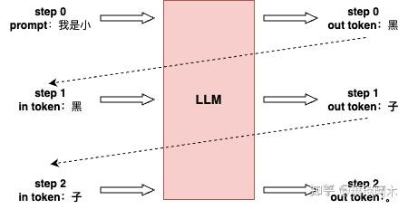
print("Generated text:", res[0]["generated_text"])

LLM推理首先输入一个预设的prompt，将其传入模型，生成首个预测的token（首字）。随后进入自回归阶段，模型依次利用前一步生成的token，预测下一个token，直至完成整个序列的生成。

Function stack

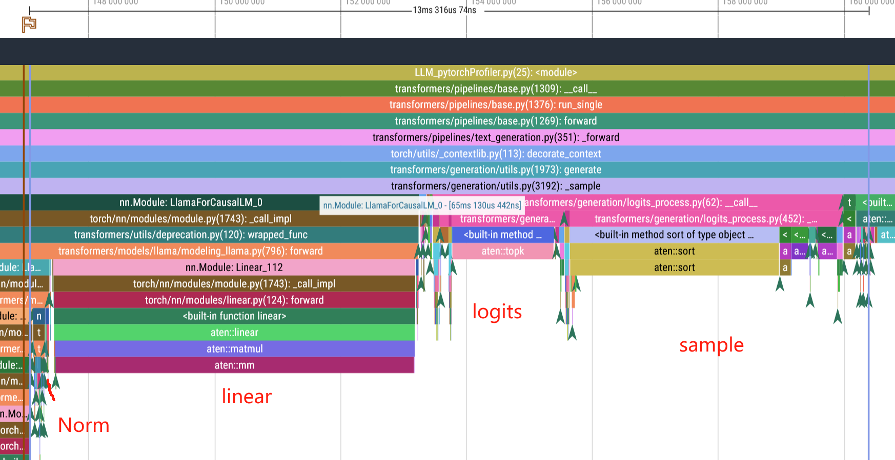
使用pytorch profiler进行观察，得到运行图

从prompt和结果那里插入

from torch.profiler import profile, record_function, ProfilerActivity
from torch.utils.tensorboard import SummaryWriter  # 用于 TensorBoard 日志

# 输入提示
prompt = "The key to life is"

# 使用 PyTorch Profiler 分析
with profile(
    activities=[ProfilerActivity.CPU],
    record_shapes=True,
    profile_memory=True,
    with_stack=True,
    on_trace_ready=torch.profiler.tensorboard_trace_handler("log_dir")  # 直接写入 TensorBoard 日志
) as prof:
    with record_function("model_inference"):
        res = pipe(prompt)

# 输出生成结果
print("Generated text:", res[0]["generated_text"])

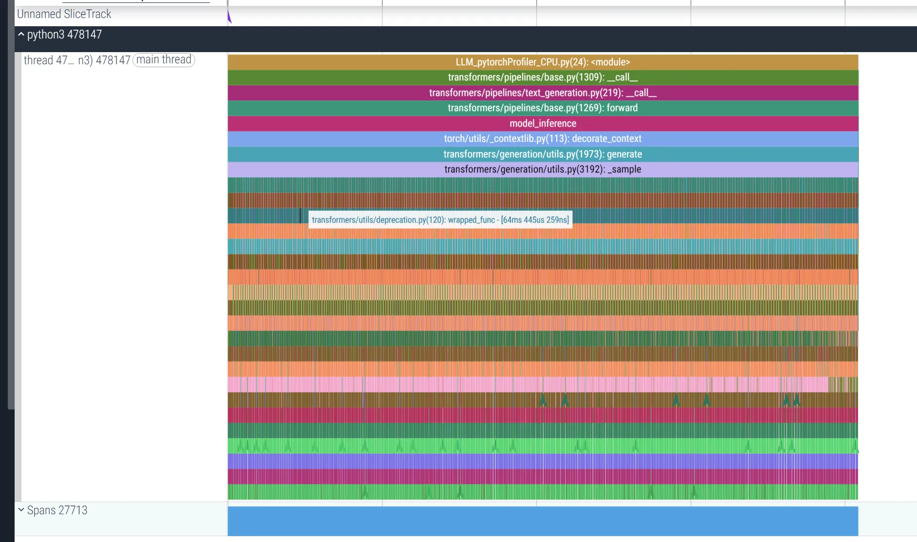
调用栈：从 pipeline.call 开始，依次调用分词器（tokenizer.encode）、生成逻辑（generate）、模型前向传播（model.forward），最后解码输出（tokenizer.decode）。

Output 层与Sample 层

图文详解LLM inference：LLM模型架构详解 - 知乎

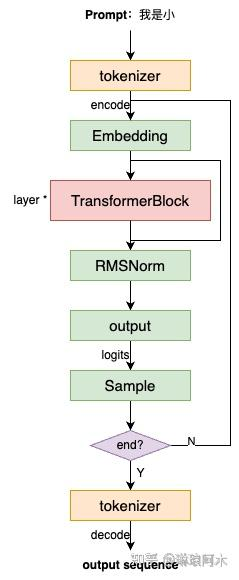
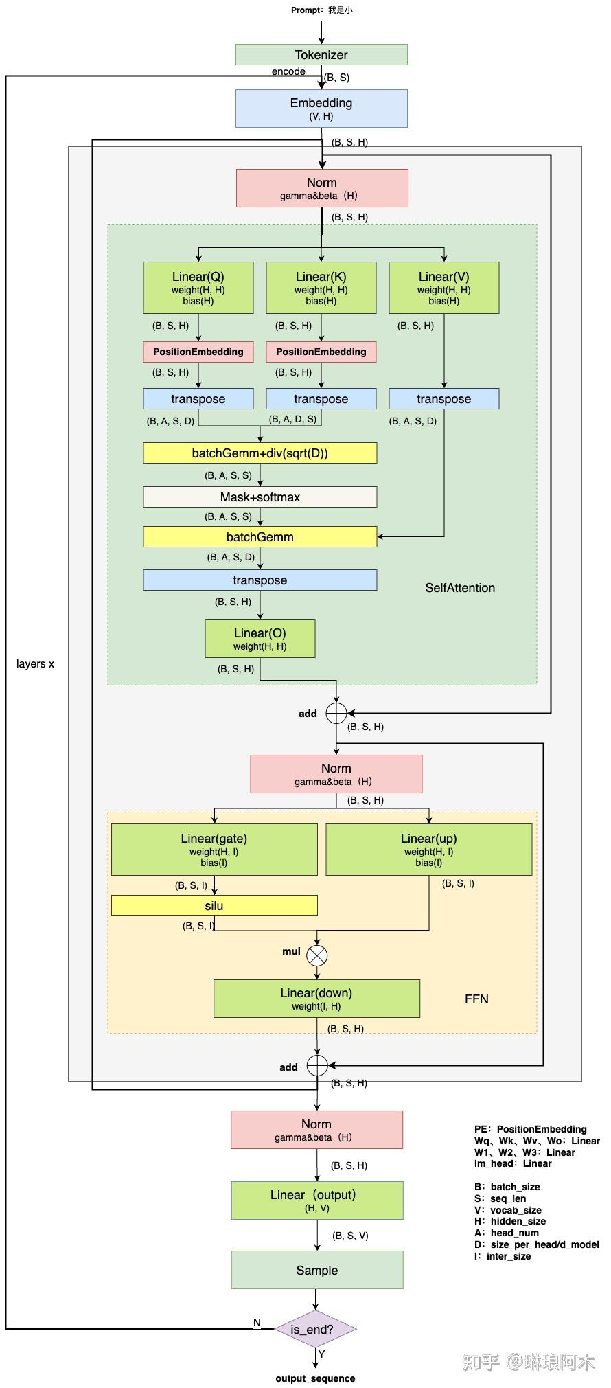
1. 模型接收预设的prompt作为输入，通过tokenizer对 prompt 进行编码（encode）为输入 token 序列。

2. 输入 token 首先经过Embedding层，转化为高维度的向量表示（通常称为词向量）。

3. 接着，这些向量依次通过多层TransformerBlock，逐层进行特征提取和信息交互，最终生成上下文相关的高维表示。

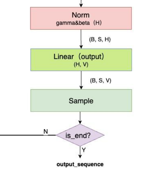
4. 然后，这些表示通过 RMSNorm层进行归一化处理，并输入到Output层，计算出预测的 logits。

5. 最后，基于 logits 对最后一个 token 进行采样，从而得到模型预测的下一个 token。

6. 重复上述过程，模型将不断地生成下一个 token，直到生成预设的end_id或检测到指定的stop_word，从而结束生成流程。

采样（sample） 有Greedy Search、Temperature Sampling、Top-k、Top-p、Beam Search等多种方式

各个block

这里边的transformer block：
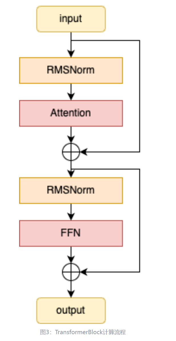
TransformerBlock 的核心组件包括两个 RMSNorm 层、一个 Attention 模块和一个 FFN（前馈神经网络）模块，其计算流程如下：

time: 4ms
Norm 200us
Attention 1.28 ms
Norm2 200us
MLP 2.3 ms

llama/llama/model.py at main · meta-llama/llama

class TransformerBlock(nn.Module):
    def __init__(self, layer_id: int, args: ModelArgs):
        """
        Initialize a TransformerBlock.

        Args:
            layer_id (int): Identifier for the layer.
            args (ModelArgs): Model configuration parameters.

        Attributes:
            n_heads (int): Number of attention heads.
            dim (int): Dimension size of the model.
            head_dim (int): Dimension size of each attention head.
            attention (Attention): Attention module.
            feed_forward (FeedForward): FeedForward module.
            layer_id (int): Identifier for the layer.
            attention_norm (RMSNorm): Layer normalization for attention output.
            ffn_norm (RMSNorm): Layer normalization for feedforward output.

        """
        super().__init__()
        self.n_heads = args.n_heads
        self.dim = args.dim
        self.head_dim = args.dim // args.n_heads
        self.attention = Attention(args)
        self.feed_forward = FeedForward(
            dim=args.dim,
            hidden_dim=4 * args.dim,
            multiple_of=args.multiple_of,
            ffn_dim_multiplier=args.ffn_dim_multiplier,
        )
        self.layer_id = layer_id
        self.attention_norm = RMSNorm(args.dim, eps=args.norm_eps)
        self.ffn_norm = RMSNorm(args.dim, eps=args.norm_eps)

    def forward(
        self,
        x: torch.Tensor,
        start_pos: int,
        freqs_cis: torch.Tensor,
        mask: Optional[torch.Tensor],
    ):
        """
        Perform a forward pass through the TransformerBlock.

        Args:
            x (torch.Tensor): Input tensor.
            start_pos (int): Starting position for attention caching.
            freqs_cis (torch.Tensor): Precomputed cosine and sine frequencies.
            mask (torch.Tensor, optional): Masking tensor for attention. Defaults to None.

        Returns:
            torch.Tensor: Output tensor after applying attention and feedforward layers.

        """
        h = x + self.attention(
            self.attention_norm(x), start_pos, freqs_cis, mask
        )
        out = h + self.feed_forward(self.ffn_norm(h)) # 图中的block在这里！！
        return out

可以看到用两行代码就干碎了。

Attention block

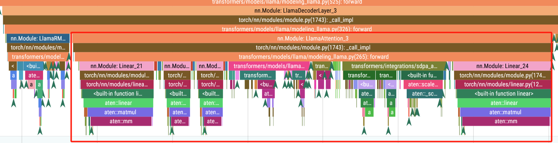
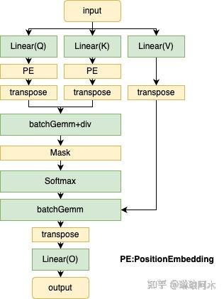
Attention 模块的核心组件主要包含Query、Key、Value 的线性变换以及输出线性投影。计算流程如下:

class Attention(nn.Module):
    """Multi-head attention module."""
    def __init__(self, args: ModelArgs):
        """
        Initialize the Attention module.

        Args:
            args (ModelArgs): Model configuration parameters.

        Attributes:
            n_kv_heads (int): Number of key and value heads.
            n_local_heads (int): Number of local query heads.
            n_local_kv_heads (int): Number of local key and value heads.
            n_rep (int): Number of repetitions for local heads.
            head_dim (int): Dimension size of each attention head.
            wq (ColumnParallelLinear): Linear transformation for queries.
            wk (ColumnParallelLinear): Linear transformation for keys.
            wv (ColumnParallelLinear): Linear transformation for values.
            wo (RowParallelLinear): Linear transformation for output.
            cache_k (torch.Tensor): Cached keys for attention.
            cache_v (torch.Tensor): Cached values for attention.

        """
        super().__init__()
        self.n_kv_heads = args.n_heads if args.n_kv_heads is None else args.n_kv_heads
        model_parallel_size = fs_init.get_model_parallel_world_size()
        self.n_local_heads = args.n_heads // model_parallel_size
        self.n_local_kv_heads = self.n_kv_heads // model_parallel_size
        self.n_rep = self.n_local_heads // self.n_local_kv_heads
        self.head_dim = args.dim // args.n_heads

        self.wq = ColumnParallelLinear(
            args.dim,
            args.n_heads * self.head_dim,
            bias=False,
            gather_output=False,
            init_method=lambda x: x,
        )
        self.wk = ColumnParallelLinear(
            args.dim,
            self.n_kv_heads * self.head_dim,
            bias=False,
            gather_output=False,
            init_method=lambda x: x,
        )
        self.wv = ColumnParallelLinear(
            args.dim,
            self.n_kv_heads * self.head_dim,
            bias=False,
            gather_output=False,
            init_method=lambda x: x,
        )
        self.wo = RowParallelLinear(
            args.n_heads * self.head_dim,
            args.dim,
            bias=False,
            input_is_parallel=True,
            init_method=lambda x: x,
        )

        self.cache_k = torch.zeros(
            (
                args.max_batch_size,
                args.max_seq_len,
                self.n_local_kv_heads,
                self.head_dim,
            )
        ).cuda()
        self.cache_v = torch.zeros(
            (
                args.max_batch_size,
                args.max_seq_len,
                self.n_local_kv_heads,
                self.head_dim,
            )
        ).cuda()

    def forward(
        self,
        x: torch.Tensor,
        start_pos: int,
        freqs_cis: torch.Tensor,
        mask: Optional[torch.Tensor],
    ):
        """
        Forward pass of the attention module.

        Args:
            x (torch.Tensor): Input tensor.
            start_pos (int): Starting position for caching.
            freqs_cis (torch.Tensor): Precomputed frequency tensor.
            mask (torch.Tensor, optional): Attention mask tensor.

        Returns:
            torch.Tensor: Output tensor after attention.

        """
        # **输入形状处理**
        bsz, seqlen, _ = x.shape

    # 1. **输入变换** - 通过三个独立的线性层将输入映射到查询（Query）、键（Key）、值（Value）空间。
        xq, xk, xv = self.wq(x), self.wk(x), self.wv(x) 

# 2. **`layout`转换
# - 将Q/K/V分别重塑为多头结构，其中：
    # - `n_local_heads`: 查询头数
    # - `n_local_kv_heads`: 键值头数（通常 ≤ 查询头数）
    # - `head_dim`: 每个头的维度
        xq = xq.view(bsz, seqlen, self.n_local_heads, self.head_dim)
        xk = xk.view(bsz, seqlen, self.n_local_kv_heads, self.head_dim)
        xv = xv.view(bsz, seqlen, self.n_local_kv_heads, self.head_dim)

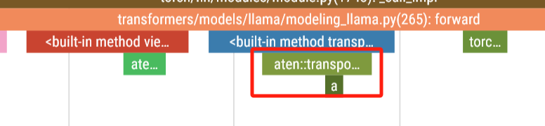
# 3. **应用旋转位置编码**
# - 使用旋转位置编码（Rotary Position Embedding）为Q/K注入位置信息，增强模型的位置感知能力。
        xq, xk = apply_rotary_emb(xq, xk, freqs_cis=freqs_cis)

# **键值缓存更新**
# - **缓存机制**：在自回归生成时，将当前步计算的键值存入缓存，避免重复计算历史token的K/V。 
# - `start_pos`表示当前处理的起始位置，适用于流式生成场景。
        self.cache_k = self.cache_k.to(xq)
        self.cache_v = self.cache_v.to(xq)

        self.cache_k[:bsz, start_pos : start_pos + seqlen] = xk
        self.cache_v[:bsz, start_pos : start_pos + seqlen] = xv

# **构建完整的注意力上下文**
        keys = self.cache_k[:bsz, : start_pos + seqlen]  # 获取历史及当前K
        values = self.cache_v[:bsz, : start_pos + seqlen]  # 获取历史及当前V

# **多头重复策略（GQA/MQA）**
# - **Grouped-Query Attention**：  repeat k/v heads if n_kv_heads < n_heads
# - `n_rep = n_local_heads // n_local_kv_heads`，表示每个KV头重复的次数。
        keys = repeat_kv(keys, self.n_rep)  # (bs, cache_len + seqlen, n_local_heads, head_dim)
        values = repeat_kv(values, self.n_rep)  # (bs, cache_len + seqlen, n_local_heads, head_dim)

# **张量转置（调整维度顺序）** - 将多头维度提前，便于后续矩阵运算。
        xq = xq.transpose(1, 2)  # (bs, n_local_heads, seqlen, head_dim)
        keys = keys.transpose(1, 2) # (bs, n_local_heads, cache_len + seqlen, head_dim)
        values = values.transpose(1, 2) # (bs, n_local_heads, cache_len + seqlen, head_dim)

# 4. **注意力得分计算** - 计算Q与K的点积，缩放因子`sqrt(d_k)`防止梯度爆炸。
        scores = torch.matmul(xq, keys.transpose(2, 3)) / math.sqrt(self.head_dim)
        # **注意力掩码处理**
        # - **因果掩码**：在解码时屏蔽未来信息，确保当前位置只能关注前面token。
        # - **填充掩码**：忽略padding token的影响。
        if mask is not None:
            scores = scores + mask  # (bs, n_local_heads, seqlen, cache_len + seqlen)
        # 5. **Softmax归一化** - 对注意力得分进行归一化，转换为概率分布。
        scores = F.softmax(scores.float(), dim=-1).type_as(xq)

        # 6. **加权求和生成上下文向量** - 使用注意力权重对Value加权求和，得到每个位置的上下文表示。
        output = torch.matmul(scores, values)  # (bs, n_local_heads, seqlen, head_dim)

        # 7. **合并多头输出** - 将多头输出拼接回原始形状，准备进行后续处理。
        output = output.transpose(1, 2).contiguous().view(bsz, seqlen, -1)

        # 8. **输出投影** - 通过线性层`wo`将多头输出映射回模型维度。
        return self.wo(output) # 线性层聚合多头信息

Attention 的计算过程如下：

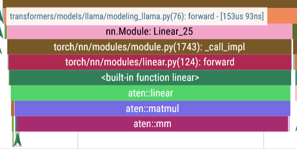
1. 输入变换：将输入的特征向量 X 通过三组独立的线性层，分别生成 Query ( Q )、Key ( K ) 和 Value ( V )，公式为： xq, xk, xv = self.wq(x), self.wk(x), self.wv(x) ​，其中， WQ ​、 WK ​、 WV ​ 是可学习的权重矩阵。

   # 1. **输入变换** - 通过三个独立的线性层将输入映射到查询（Query）、键（Key）、值（Value）空间。
       xq, xk, xv = self.wq(x), self.wk(x), self.wv(x) 

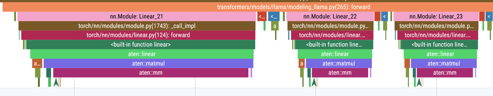
Matmul 1: 200us
Matmul 2: 71us
Matmul 3: 70us

2. layout转换： 将 Query ( Q )、Key ( K ) 和 Value ( V )的的张量布局由[batch_size,seq_len,head_num,d_model]转为 [batch_size,head_num,seq_len,d_model]，这种布局转换是为了适应多头注意力机制的计算需求，将每个头的查询、键和值的维度重新排列，使得计算能够并行处理不同头部的注意力权重，同时提高计算效率。

3. 位置编码：将位置信息加入到 Q 和 K 向量中，以便模型能够捕捉到序列中元素的顺序关系。通过对 Q 和 K 进行位置编码，Transformer模型可以理解输入序列中元素的相对或绝对位置，从而在自注意力机制中更好地处理序列顺序的依赖性。

4. 计算注意力得分：
   通过点积操作计算 Query 和 Key 之间的相似度，获得注意力得分矩阵： 
   

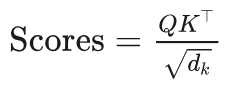
   这里， dk ​ 是 Key 的特征维度，用于缩放防止数值过大。

5. 归一化得分：
   对得分矩阵应用 Softmax 函数，将其归一化为概率分布： Attention Weights=Softmax(Scores)

6. 加权求和：
   使用归一化后的注意力权重对 Value 矩阵进行加权求和，生成上下文表示： Attention Output=Attention Weights⋅V

7. layout转换：将Attention Output 的张量布局从[batch_size,head_num,seq_len,d_model]转为[batch_size,seq_len,head_num,d_model]，这一转换是为了恢复原始序列的顺序，并将多头注意力的输出按序列长度排列，以便后续操作（如拼接或线性变换）能够正确地处理每个头的输出信息。

8. 线性投影：
   将多头注意力的输出拼接后，输入线性层进行投影，生成最终的注意力输出： Final Output=Concat(Head1,Head2,…)WO ，​其中， Wo ​ 是线性投影的权重矩阵。

通过这一过程，Attention 模块能够动态聚焦输入序列中不同位置的重要信息，建模长距离依赖关系。

核心特点解析：

1. 高效缓存机制
   • 通过维护cache_k和cache_v，避免在自回归生成时重复计算历史token的K/V，显著提升推理效率。
2. 灵活的多头策略
   • 支持多查询注意力（MQA）和分组查询注意力（GQA），通过repeat_kv实现KV头的复用，平衡计算效率和模型表现。
3. 旋转位置编码（RoPE）
   • 通过绝对位置编码实现相对位置感知，增强模型对位置关系的建模能力。
4. 并行计算优化
   • 通过矩阵运算并行处理整个序列，充分利用GPU加速。
     此实现通过结合现代Transformer模型的多种优化技术，在保证模型表现的同时提升了推理效率。

在使用huggingface中llama3的源码：

class LlamaAttention(nn.Module):
    """Multi-headed attention from 'Attention Is All You Need' paper"""

    def __init__(self, config: LlamaConfig, layer_idx: int):
        super().__init__()
        self.config = config
        self.layer_idx = layer_idx
        self.head_dim = getattr(config, "head_dim", config.hidden_size // config.num_attention_heads)
        self.num_key_value_groups = config.num_attention_heads // config.num_key_value_heads
        self.scaling = self.head_dim**-0.5
        self.attention_dropout = config.attention_dropout
        self.is_causal = True

        self.q_proj = nn.Linear(
            config.hidden_size, config.num_attention_heads * self.head_dim, bias=config.attention_bias
        )
        self.k_proj = nn.Linear(
            config.hidden_size, config.num_key_value_heads * self.head_dim, bias=config.attention_bias
        )
        self.v_proj = nn.Linear(
            config.hidden_size, config.num_key_value_heads * self.head_dim, bias=config.attention_bias
        )
        self.o_proj = nn.Linear(
            config.num_attention_heads * self.head_dim, config.hidden_size, bias=config.attention_bias
        )

    def forward(
        self,
        hidden_states: torch.Tensor,
        position_embeddings: Tuple[torch.Tensor, torch.Tensor],
        attention_mask: Optional[torch.Tensor],
        past_key_value: Optional[Cache] = None,
        cache_position: Optional[torch.LongTensor] = None,
        **kwargs: Unpack[FlashAttentionKwargs],
    ) -> Tuple[torch.Tensor, Optional[torch.Tensor], Optional[Tuple[torch.Tensor]]]:
        input_shape = hidden_states.shape[:-1]
        hidden_shape = (*input_shape, -1, self.head_dim)

# // load QKV
        query_states = self.q_proj(hidden_states).view(hidden_shape).transpose(1, 2)
        key_states = self.k_proj(hidden_states).view(hidden_shape).transpose(1, 2)
        value_states = self.v_proj(hidden_states).view(hidden_shape).transpose(1, 2)

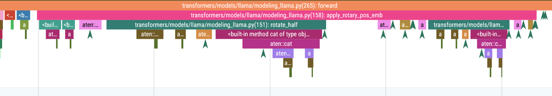
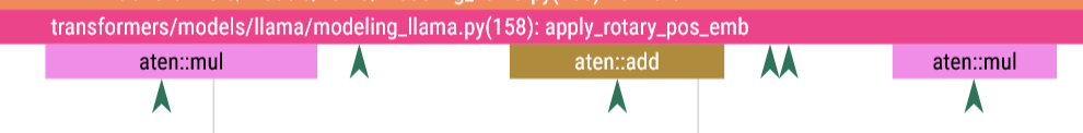
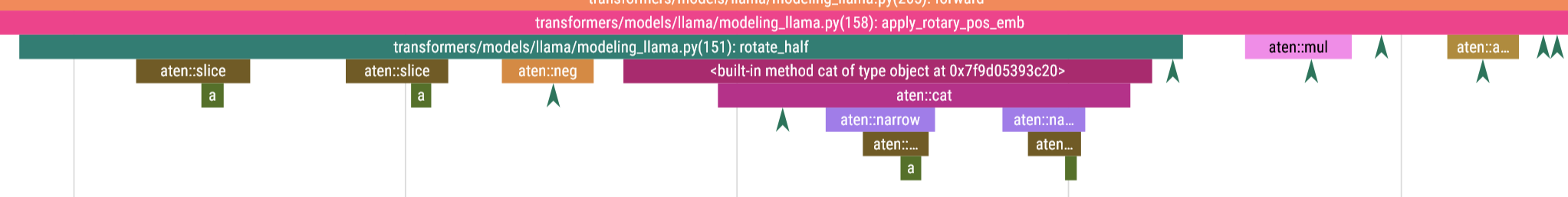
# ROPE
        cos, sin = position_embeddings
        query_states, key_states = apply_rotary_pos_emb(query_states, key_states, cos, sin)

# KV cache
        if past_key_value is not None:
            # sin and cos are specific to RoPE models; cache_position needed for the static cache
            cache_kwargs = {"sin": sin, "cos": cos, "cache_position": cache_position}
            key_states, value_states = past_key_value.update(key_states, value_states, self.layer_idx, cache_kwargs)

# ATTENTION
        attention_interface: Callable = eager_attention_forward

        if self.config._attn_implementation != "eager":
            if self.config._attn_implementation == "sdpa" and kwargs.get("output_attentions", False):
                logger.warning_once(
                    "`torch.nn.functional.scaled_dot_product_attention` does not support `output_attentions=True`. Falling back to "
                    'eager attention. This warning can be removed using the argument `attn_implementation="eager"` when loading the model.'
                )
            else:
                attention_interface = ALL_ATTENTION_FUNCTIONS[self.config._attn_implementation]

        attn_output, attn_weights = attention_interface(
            self,
            query_states,
            key_states,
            value_states,
            attention_mask,
            dropout=0.0 if not self.training else self.attention_dropout,
            scaling=self.scaling,
            **kwargs,
        )

        attn_output = attn_output.reshape(*input_shape, -1).contiguous()
        attn_output = self.o_proj(attn_output)
        return attn_output, attn_weights

其实跟llama自己的实现大差不差。

这段代码定义了一个基于 Llama 模型的多头注意力机制（Multi-Head Attention）的 PyTorch 实现，参考了《Attention Is All You Need》论文。以下是对其推理过程（即 forward 方法）的详细解读，结合代码逐步分析其工作原理和关键点：

---

1. 代码结构概述

LlamaAttention 是一个 nn.Module，实现了一个 Transformer 的多头注意力层。它支持：

• 分组查询注意力（Grouped-Query Attention, GQA）：通过 num_key_value_groups 实现，减少键值对头的数量以优化计算。
• 旋转位置编码（Rotary Positional Embedding, RoPE）：通过 apply_rotary_pos_emb 融入位置信息。
• 键值缓存（Key-Value Cache）：用于加速自回归推理（如生成任务）。
• 多种注意力实现：支持 eager（默认逐行计算）、sdpa（PyTorch 的 scaled_dot_product_attention）或 flash（如 FlashAttention 优化）。

推理过程发生在 forward 方法中，输入包括：

• hidden_states：输入的隐藏状态张量，形状为 (batch_size, seq_len, hidden_size)。
• position_embeddings：RoPE 的余弦（cos）和正弦（sin）位置编码。
• attention_mask：可选的掩码，用于屏蔽某些位置（如填充 token 或因果注意力）。
• past_key_value：键值缓存，用于自回归推理。
• cache_position：缓存的位置索引。
• kwargs：额外参数（如 FlashAttention 的配置）。

输出为：

• attn_output：注意力计算后的输出张量，形状为 (batch_size, seq_len, hidden_size)。
• attn_weights：注意力权重（可选，训练时可能用到）。

---

2. 推理过程逐行解读

输入处理

input_shape = hidden_states.shape[:-1]  # (batch_size, seq_len)
hidden_shape = (*input_shape, -1, self.head_dim)  # (batch_size, seq_len, num_heads, head_dim)

• 提取输入张量的形状，input_shape 保存 batch_size 和 seq_len，忽略最后一维（hidden_size）。
• 定义 hidden_shape，用于将张量重塑为多头格式，其中 -1 会被替换为 num_attention_heads 或 num_key_value_heads。

线性投影

        self.q_proj = nn.Linear(
            config.hidden_size, config.num_attention_heads * self.head_dim, bias=config.attention_bias
        )
        self.k_proj = nn.Linear(
            config.hidden_size, config.num_key_value_heads * self.head_dim, bias=config.attention_bias
        )
        self.v_proj = nn.Linear(
            config.hidden_size, config.num_key_value_heads * self.head_dim, bias=config.attention_bias
        )

query_states = self.q_proj(hidden_states).view(hidden_shape).transpose(1, 2)
key_states = self.k_proj(hidden_states).view(hidden_shape).transpose(1, 2)
value_states = self.v_proj(hidden_states).view(hidden_shape).transpose(1, 2)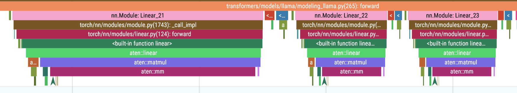

• 投影：通过线性层 q_proj、k_proj 和 v_proj，将输入的 hidden_states 分别映射到查询（Query）、键（Key）和值（Value）张量。
  • 查询张量的输出维度：num_attention_heads * head_dim。
  • 键和值张量的输出维度：num_key_value_heads * head_dim（GQA 可能使 num_key_value_heads 小于 num_attention_heads）。
• 重塑：使用 view(hidden_shape) 将张量重塑为 (batch_size, seq_len, num_heads, head_dim)，其中 num_heads 对应于注意力头数。
• 转置：通过 transpose(1, 2) 将张量变为 (batch_size, num_heads, seq_len, head_dim)，方便后续按头并行计算注意力。
  

Matmul 1: 200us
Matmul 2: 71us
Matmul 3: 70us

应用旋转位置编码（RoPE）

cos, sin = position_embeddings
query_states, key_states = apply_rotary_pos_emb(query_states, key_states, cos, sin)

• position_embeddings 是一个包含余弦和正弦值的元组，用于 RoPE。
• apply_rotary_pos_emb 函数将位置信息融入 query_states 和 key_states，通过旋转操作（基于正弦和余弦）为每个 token 添加位置依赖性。
• 注意：value_states 不应用 RoPE，因为值张量不直接依赖位置信息。
  
  200us

键值缓存（Key-Value Cache）

if past_key_value is not None:
    cache_kwargs = {"sin": sin, "cos": cos, "cache_position": cache_position}
    key_states, value_states = past_key_value.update(key_states, value_states, self.layer_idx, cache_kwargs)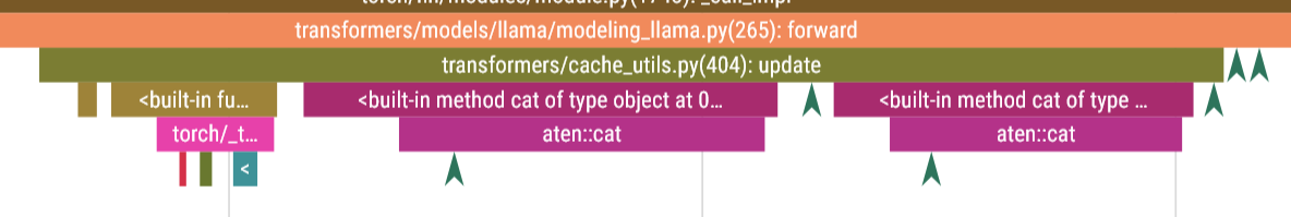

Time: 50us

• 作用：在自回归推理（如语言生成）中，键值缓存存储之前时间步的 key_states 和 value_states，避免重复计算。
• 更新缓存：past_key_value.update 将当前时间步的 key_states 和 value_states 追加到缓存中，并返回更新后的键值张量。
• 参数：
  • sin 和 cos：用于 RoPE 的位置编码。
  • cache_position：指示当前 token 在序列中的位置。
  • layer_idx：标识当前注意力层的索引。
• 推理优化：在生成任务中，模型通常只处理最新 token，缓存允许快速访问历史信息，显著降低计算量。

选择注意力实现

attention_interface: Callable = eager_attention_forward
if self.config._attn_implementation != "eager":
    if self.config._attn_implementation == "sdpa" and kwargs.get("output_attentions", False):
        logger.warning_once(...)
    else:
        attention_interface = ALL_ATTENTION_FUNCTIONS[self.config._attn_implementation]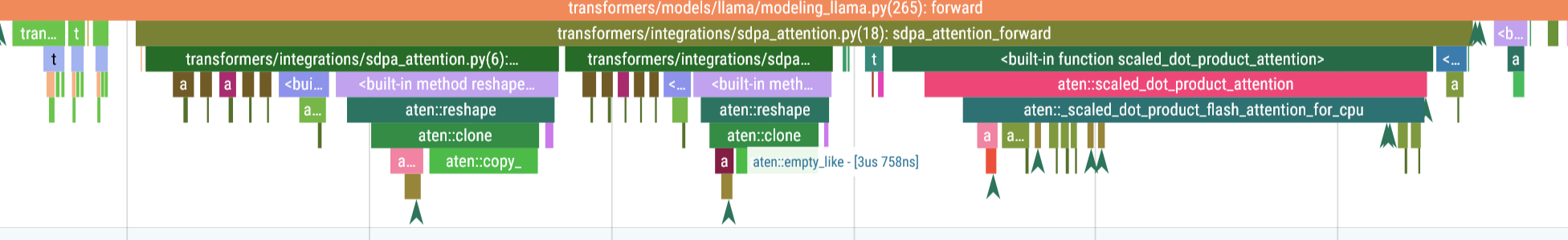

20 us

• 根据 config._attn_implementation，选择注意力计算方式：
  • eager：逐行实现的标准注意力，适合调试或需要输出注意力权重。
  • sdpa：使用 PyTorch 的 scaled_dot_product_attention，性能更高，但不支持 output_attentions=True。
  • flash：使用 FlashAttention 或类似优化，适合大规模模型，效率最高。
• 如果选择了 sdpa 但要求输出注意力权重，会回退到 eager 并发出警告。

计算注意力

attn_output, attn_weights = attention_interface(
    self,
    query_states,
    key_states,
    value_states,
    attention_mask,
    dropout=0.0 if not self.training else self.attention_dropout,
    scaling=self.scaling,
    **kwargs,
)

Scaled Dot-product Attention：276 us

• 核心计算：调用选定的 attention_interface 执行注意力机制：
  • 缩放点积：计算 Q @ K^T / sqrt(head_dim)，得到注意力分数（self.scaling = head_dim**-0.5 用于稳定梯度）。
  • 掩码：应用 attention_mask（如因果掩码，防止未来 token 影响当前 token）。
  • Softmax：将注意力分数归一化为权重。
  • 加权求和：用注意力权重加权 value_states，得到每头的输出。
• Dropout：推理时（self.training=False）禁用 dropout，训练时根据 attention_dropout 应用。
• 输出：
  • attn_output：形状为 (batch_size, num_heads, seq_len, head_dim)，表示注意力结果。
  • attn_weights：注意力权重（可能为 None，依赖实现和配置）。

输出投影与重塑

        self.o_proj = nn.Linear(
            config.num_attention_heads * self.head_dim, config.hidden_size, bias=config.attention_bias
        )

attn_output = attn_output.reshape(*input_shape, -1).contiguous()
attn_output = self.o_proj(attn_output)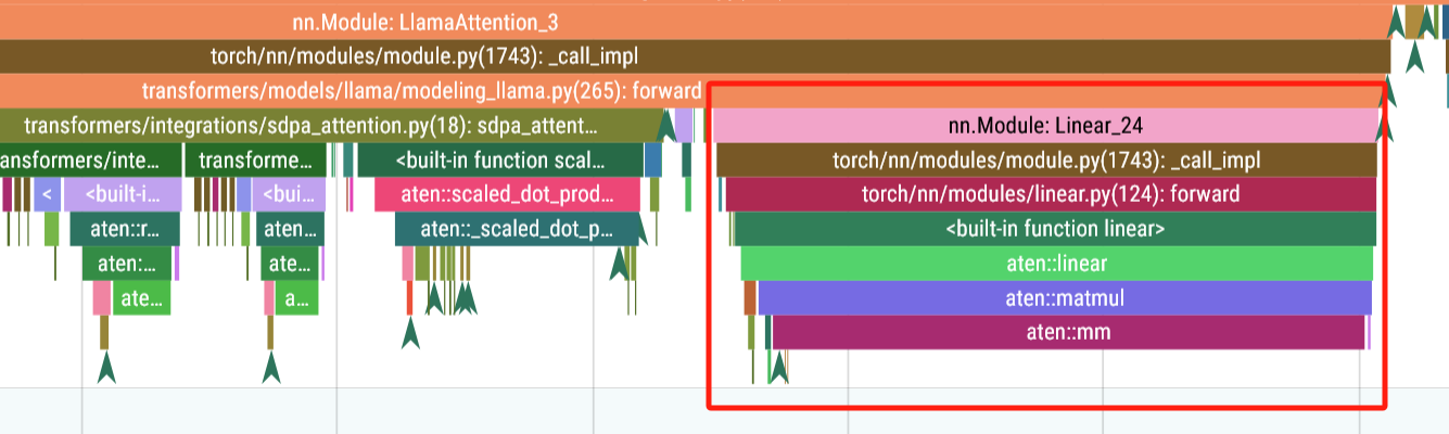

time: 263us

• 重塑：将 attn_output 从 (batch_size, num_heads, seq_len, head_dim) 变回 (batch_size, seq_len, num_attention_heads * head_dim)。
• 投影：通过 o_proj 线性层将注意力输出映射回 hidden_size 维度，得到最终输出，形状为 (batch_size, seq_len, hidden_size)。
• contiguous：确保张量在内存中连续，优化后续操作。

返回结果

return attn_output, attn_weights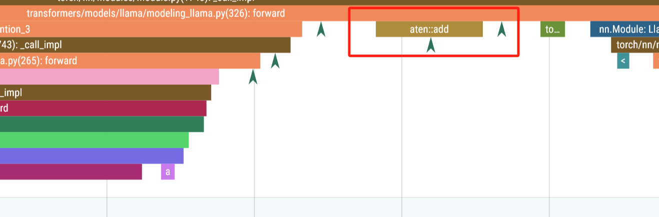

• 返回 attn_output（注意力层输出）和 attn_weights（注意力权重，若计算则返回，否则可能为 None）。

---

3. 推理中的关键优化

1. 分组查询注意力（GQA）：

   • num_key_value_groups 定义了查询头与键值头之间的分组比例。
   • 减少 num_key_value_heads（键值对头数）降低内存和计算开销，同时保持 num_attention_heads（查询头数）以保留表达能力。
   • 在推理中，这显著减少了键值缓存的内存占用。

2. 键值缓存：

   • 在自回归推理中，缓存历史键值对避免重复计算。
   • 每次只处理最新 token，缓存将历史信息与当前输入拼接，推理时间从 O(seq_len^2) 降为 O(seq_len)。

3. 旋转位置编码（RoPE）：

   • RoPE 通过旋转操作融入位置信息，无需显式位置嵌入，减少参数量。
   • 在推理中，sin 和 cos 可预计算，动态应用于当前 token。

4. 高效注意力实现：

   • flash 模式（如 FlashAttention）通过融合操作减少 GPU 内存读写，加速推理。
   • sdpa 利用 PyTorch 优化的内核，适合中小规模模型。
   • 选择合适的实现根据硬件和模型规模平衡速度与功能（如是否需要 attn_weights）。

5. 因果注意力：

   • self.is_causal = True 表明这是一个自回归模型，推理时通过 attention_mask 确保当前 token 只关注之前 token。

---

4. 推理性能分析

• 计算复杂度：
  • 投影层（q_proj, k_proj, v_proj, o_proj）：O(seq_len * hidden_size^2)。
  • 注意力计算：O(seq_len^2 head_dim num_heads)（无缓存），或 O(seq_len head_dim num_heads)（有缓存）。
  • GQA 进一步减少键值计算量。
• 内存需求：
  • 键值缓存：O(seq_len num_key_value_heads head_dim * num_layers)。
  • FlashAttention 减少中间张量的内存占用。
• 瓶颈：
  • 长序列推理时，缓存内存可能成为瓶颈。
  • 注意力计算（尤其是 eager 模式）可能较慢，推荐 flash 或 sdpa。

---

LlamaAttention 的推理过程高效地实现了多头注意力，结合 GQA、RoPE 和键值缓存优化了自回归生成任务的性能。其核心步骤包括投影、位置编码、注意力计算和输出投影，支持多种高效实现（如 FlashAttention）。在推理中，缓存和 GQA 是关键优化点，显著降低计算和内存开销，适合大规模语言模型的部署。

FFN

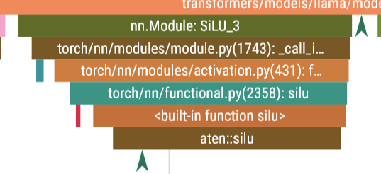
Silu

matmul

llama/llama/model.py at main · meta-llama/llama

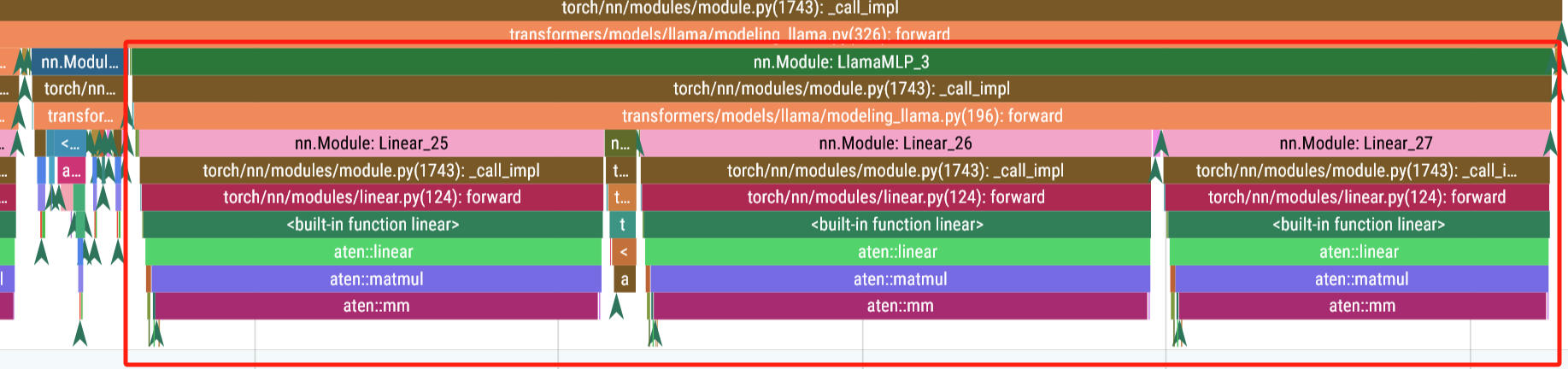
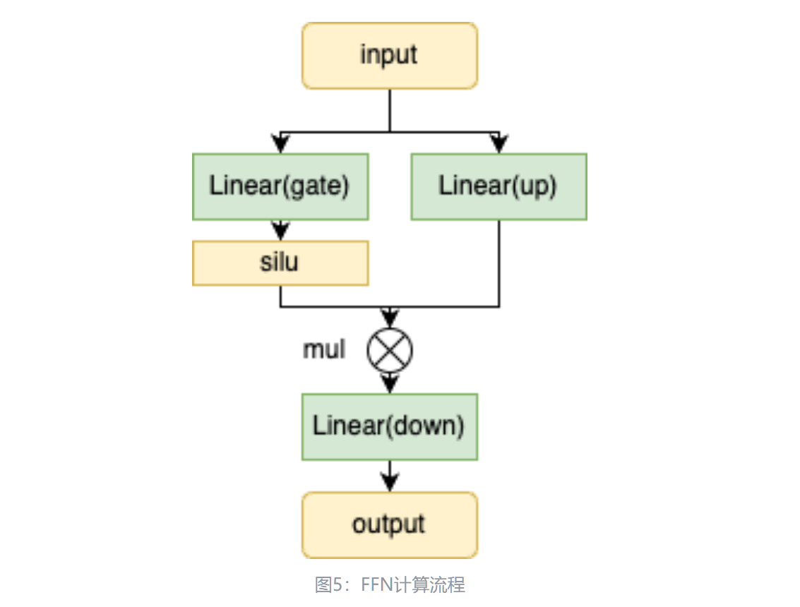
首先，输入通过两个全连接层——gate和up进行初步变换，其中gate的输出经过激活函数（silu）进行非线性变换，与up的输出做点乘，最后再通过down全连接层进行进一步处理。FFN模块的作用是增强模型的表达能力，从而在Transformer架构中捕捉更复杂的特征。

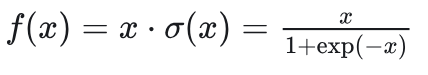
silu 公式：

class FeedForward(nn.Module):
    def __init__(
        self,
        dim: int,
        hidden_dim: int,
        multiple_of: int,
        ffn_dim_multiplier: Optional[float],
    ):
        """
        Initialize the FeedForward module.

        Args:
            dim (int): Input dimension.
            hidden_dim (int): Hidden dimension of the feedforward layer.
            multiple_of (int): Value to ensure hidden dimension is a multiple of this value.
            ffn_dim_multiplier (float, optional): Custom multiplier for hidden dimension. Defaults to None.

        Attributes:
            w1 (ColumnParallelLinear): Linear transformation for the first layer.
            w2 (RowParallelLinear): Linear transformation for the second layer.
            w3 (ColumnParallelLinear): Linear transformation for the third layer.

        """
        super().__init__()
        hidden_dim = int(2 * hidden_dim / 3)
        # custom dim factor multiplier
        if ffn_dim_multiplier is not None:
            hidden_dim = int(ffn_dim_multiplier * hidden_dim)
        hidden_dim = multiple_of * ((hidden_dim + multiple_of - 1) // multiple_of)

        self.w1 = ColumnParallelLinear(
            dim, hidden_dim, bias=False, gather_output=False, init_method=lambda x: x
        )
        self.w2 = RowParallelLinear(
            hidden_dim, dim, bias=False, input_is_parallel=True, init_method=lambda x: x
        )
        self.w3 = ColumnParallelLinear(
            dim, hidden_dim, bias=False, gather_output=False, init_method=lambda x: x
        )

    def forward(self, x):
        return self.w2(F.silu(self.w1(x)) * self.w3(x))

FeedForward 是一个 nn.Module，实现了一个前馈网络，常见于 Transformer 的每个注意力层之后。它的主要特点包括：

• SwiGLU 激活：结合 SiLU（Swish）激活函数和门控机制，增强非线性表达能力。
• 并行线性层：使用 ColumnParallelLinear 和 RowParallelLinear，支持模型并行（如张量并行），适合分布式训练。
• 动态隐藏维度：通过 multiple_of 和 ffn_dim_multiplier 调整隐藏层维度，确保高效计算和内存对齐。

代码由两部分组成：

1. init：初始化模块，定义线性层和隐藏维度。
2. forward：定义前向传播逻辑，执行 MLP 计算。

参数

def __init__(
    self,
    dim: int,                    # 输入维度
    hidden_dim: int,            # 隐藏层维度（初始值）
    multiple_of: int,           # 确保隐藏维度是该值的倍数
    ffn_dim_multiplier: Optional[float],  # 可选的隐藏维度缩放因子
):

• dim：输入和输出的维度，通常等于 Transformer 的 hidden_size（如 4096）。
• hidden_dim：隐藏层的初始维度，通常较大（如 4 * dim）。
• multiple_of：用于调整隐藏维度，使其成为某个值的倍数（优化内存对齐和计算效率）。
• ffn_dim_multiplier：可选的缩放因子，用于自定义隐藏维度。

隐藏维度调整

hidden_dim = int(2 * hidden_dim / 3)
if ffn_dim_multiplier is not None:
    hidden_dim = int(ffn_dim_multiplier * hidden_dim)
hidden_dim = multiple_of * ((hidden_dim + multiple_of - 1) // multiple_of)

• 初始缩放：hidden_dim = int(2 * hidden_dim / 3)，将输入的 hidden_dim 缩减到原来的 2/3。这可能是为了适配 SwiGLU 的门控机制，降低计算量。
• 自定义缩放：如果提供了 ffn_dim_multiplier，则进一步按该因子调整 hidden_dim。
• 对齐调整：通过 multiple_of * ((hidden_dim + multiple_of - 1) // multiple_of)，确保 hidden_dim 是 multiple_of 的倍数。这种对齐优化了 GPU/TPU 上的内存访问和计算效率（例如，适配 SIMD 指令或缓存行）。

线性层定义

self.w1 = ColumnParallelLinear(
    dim, hidden_dim, bias=False, gather_output=False, init_method=lambda x: x
)
self.w2 = RowParallelLinear(
    hidden_dim, dim, bias=False, input_is_parallel=True, init_method=lambda x: x
)
self.w3 = ColumnParallelLinear(
    dim, hidden_dim, bias=False, gather_output=False, init_method=lambda x: x
)

• 线性层：
  • w1：从 dim 映射到 hidden_dim，用于计算 SwiGLU 的主路径。
  • w3：从 dim 映射到 hidden_dim，用于计算 SwiGLU 的门控路径。
  • w2：从 hidden_dim 映射回 dim，生成最终输出。
• 并行特性：
  • ColumnParallelLinear：输入按列分割，适合张量并行，每个进程处理部分输出维度（hidden_dim）。
  • RowParallelLinear：输入按行分割（hidden_dim），输出在进程间聚合，恢复 dim 维度。
  • gather_output=False（w1, w3）：输出保留分割状态，减少通信开销。
  • input_is_parallel=True（w2）：输入已经是并行分割的，匹配 w1 和 w3 的输出。
• 无偏置：bias=False，减少参数量，依赖归一化层（如 LayerNorm）处理偏移。
• 初始化：init_method=lambda x: x，保留输入权重（可能在外部统一初始化）。

FeedForward 模块中的三个线性层（w1, w2, w3）执行的实际运算是矩阵乘法，这是 PyTorch 中 nn.Linear（及其并行变体 ColumnParallelLinear 和 RowParallelLinear）的核心操作。

ColumnParallelLinear

w1_out = x @ w1_weight^T

w3_out = x @ w3_weight^T

• 权重矩阵按 hidden_dim 维度分割到多个设备。
• 每个设备计算部分输出维度，输出仍为 (batch_size * seq_len, hidden_dim)，但分割存储（gather_output=False）。

RowParallelLinear

w2_out = gate_out @ w2_weight^T

• 输入 gate_out 按 hidden_dim 维度分割（与 w1 和 w3 的输出匹配，input_is_parallel=True）。
• 每个设备计算部分矩阵乘法，结果按 dim 维度聚合，生成完整的 (batch_size * seq_len, dim)。

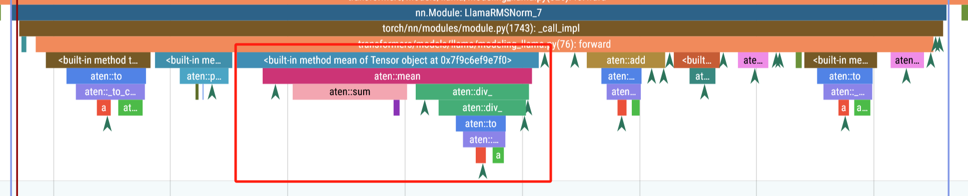
RMSNorm

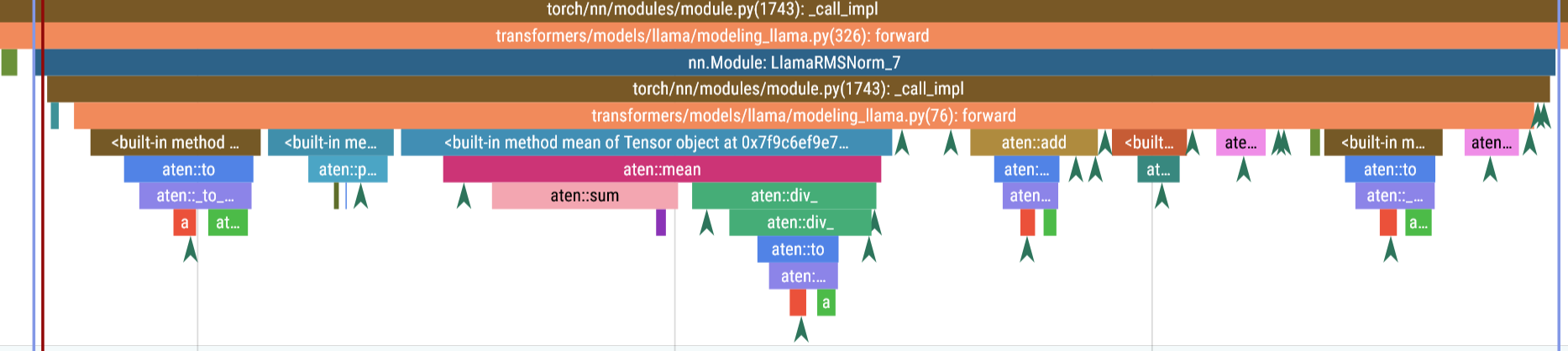
159us

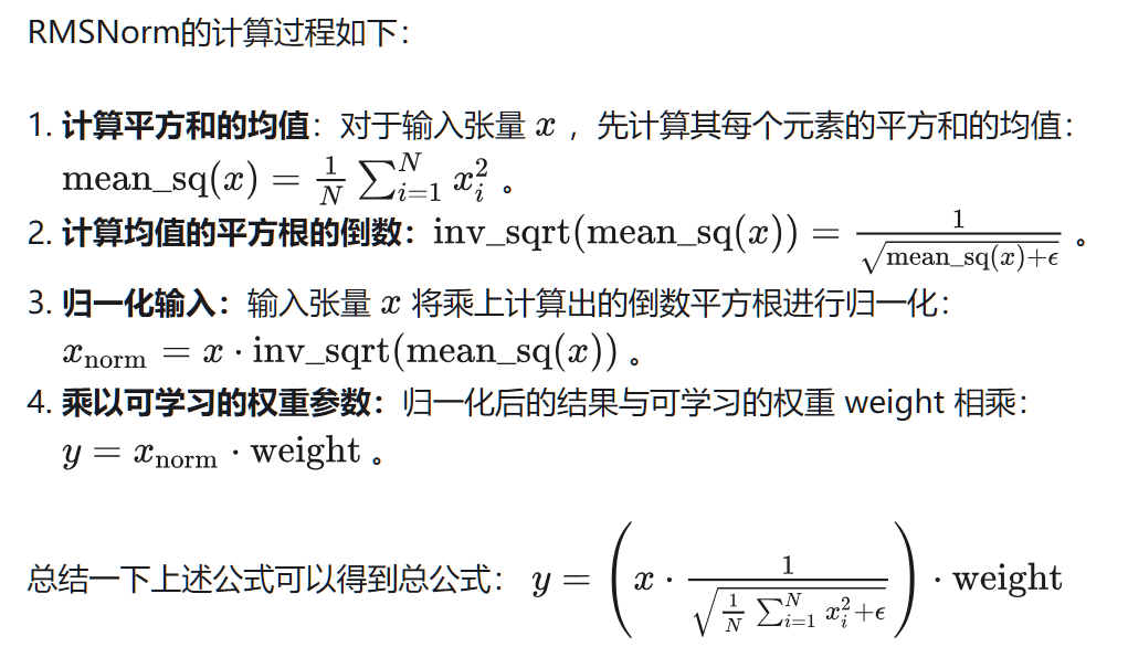
1. 计算均值
   

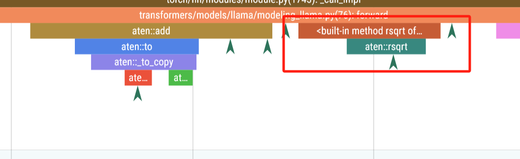
2. 平方根倒数
   

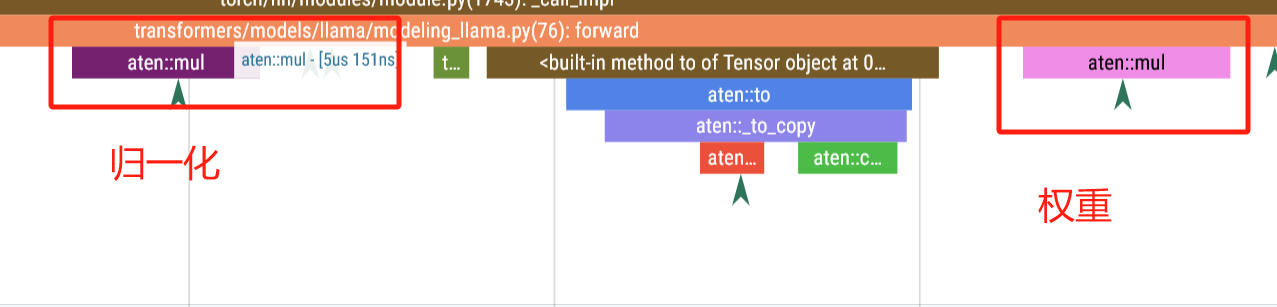
3. 归一化

4. 权重
   

class RMSNorm(torch.nn.Module):
    def __init__(self, dim: int, eps: float = 1e-6):
        super().__init__()
        self.eps = eps
        self.weight = nn.Parameter(torch.ones(dim))

    def _norm(self, x):
        return x * torch.rsqrt(x.pow(2).mean(-1, keepdim=True) + self.eps)

    def forward(self, x):
        output = self._norm(x.float()).type_as(x)
        return output * self.weight

整体结构

为了简化讨论，这里我们采用了MHA（多头注意力）结构的模型作为示例。对于GQA（分组注意力）、MQA（混合注意力）等其他变体模型，也可以通过类似的方法进行类比和分析。

为了简化图示表达，我们对大模型推理过程中常见的张量形状进行了简化表示：

• Batch Size (B)：表示每次推理中处理的样本数量。
• Sequence Length (S)：表示每个样本的序列长度，通常是文本的单词或字符数。
• Hidden Size (H)：表示隐藏层的维度，通常与模型的复杂度相关。
• Vocabulary Size (V)：表示模型词汇表的大小，通常决定了词嵌入的维度。
• Number of Attention Heads (A)：表示每层自注意力机制的头数，影响模型的计算量。
  

Output 层与Sample 层

掌握一个模型的架构及优化方法，可以通过类比快速理解并迁移到其他模型上。

要深入了解大型语言模型（LLM）在 CPU 端的推理加速，以及整个系统的调用栈，分析 transformers 库的源码是一个很好的起点，以下是逐步解析调用栈和建议从哪里开始看源码的指南：

---

1. 理解 pipeline 的调用栈

在你的代码中，pipe = pipeline(...) 和 res = pipe(prompt) 是核心调用点。以下是 pipeline 的高层调用流程：

• pipeline 初始化 (pipeline("text-generation", ...)):

  • pipeline 会根据任务（text-generation）加载模型和分词器（tokenizer）。
  • 它会调用 AutoModelForCausalLM（或其他适配模型类）来加载 meta-llama/Llama-3.2-1B 模型。
  • 模型会被加载到指定设备（device_map="auto"），并根据 torch_dtype（如 bfloat16）进行优化。
  • 相关的配置（如 max_new_tokens）会被传递到生成逻辑中。

• 推理过程 (pipe(prompt)):

  • 输入 prompt 被分词器编码为 token IDs。
  • 编码后的输入被送入模型进行前向传播，生成 logits。
  • 生成逻辑（通常是贪婪搜索、束搜索或采样）根据 logits 选择下一个 token。
  • 重复生成直到达到 max_new_tokens 或遇到终止条件。
  • 最后，生成的 token IDs 被解码为文本输出。

整个过程涉及以下组件：

• 分词器：将文本转为 token IDs。
• 模型：执行前向传播，生成 logits。
• 生成逻辑：基于 logits 选择 token。
• 设备管理：CPU 或 GPU 的张量运算。

---

2. 调用栈的关键点

以下是 transformers 库中与你的代码相关的调用栈（基于 pipeline 的 text-generation 任务）：

1. pipeline 初始化:

   • 源码位置：transformers/pipelines/__init__.py
     • pipeline 函数会根据任务类型（text-generation）选择合适的 pipeline 类（TextGenerationPipeline）。
   • 源码位置：transformers/pipelines/text_generation.py
     • TextGenerationPipeline 初始化时加载模型（AutoModelForCausalLM）和分词器（AutoTokenizer）。
   • 源码位置：transformers/models/auto/auto_factory.py
     • AutoModelForCausalLM.from_pretrained(model_id) 加载预训练模型。
   • 源码位置：transformers/modeling_utils.py
     • from_pretrained 方法处理模型权重加载、设备映射（device_map）和数据类型（torch_dtype）。

2. 推理调用 (pipe(prompt)):

   • 源码位置：transformers/pipelines/text_generation.py
     • TextGenerationPipeline.__call__ 方法处理输入 prompt，调用分词器编码和模型生成。
   • 源码位置：transformers/generation/utils.py
     • generate 方法实现生成逻辑（如贪婪搜索、采样等）。
     • 它调用模型的 forward 方法（前向传播）生成 logits。
   • 源码位置：transformers/models/llama/modeling_llama.py
     • 对于 Llama-3.2-1B，LlamaForCausalLM.forward 实现前向传播，计算注意力机制和 MLP 的输出。
   • 源码位置：torch/nn/modules/*
     • PyTorch 的底层模块（如线性层、注意力机制）在 CPU 上执行张量运算。

3. 分词器:

   • 源码位置：transformers/tokenization_utils_base.py
     • 分词器的 encode 和 decode 方法处理文本到 token 的转换。
   • 对于 Llama 模型，分词器通常基于 sentencepiece 或自定义实现。

4. 设备和数据类型管理:

   • 源码位置：transformers/utils/generic.py 和 accelerate 库
     • device_map="auto" 使用 accelerate 库来分配模型权重到 CPU 或 GPU。
   • 源码位置：torch/*
     • PyTorch 管理张量的数据类型（bfloat16）和设备（CPU）。

---

3. 从哪里开始看源码

为了研究 LLM 在 CPU 端的推理加速，建议按照以下步骤逐步阅读源码，并关注与性能优化的相关部分：

步骤 1：从 pipeline 入手

• 文件：transformers/pipelines/text_generation.py
  • 查看 TextGenerationPipeline 的 __call__ 方法，了解如何调用分词器和模型。
  • 重点关注 _forward 和 postprocess 方法，它们处理模型推理和输出解码。
• 为什么：pipeline 是高层接口，理解它可以快速把握推理流程的全貌。

步骤 2：深入生成逻辑

• 文件：transformers/generation/utils.py
  • 查看 GenerationMixin.generate 方法，这是生成 token 的核心逻辑。
  • 关注 greedy_search 或 sample 方法（取决于你的生成配置），它们控制如何从 logits 中选择 token。
• 为什么：生成逻辑涉及多次模型调用，优化这里可以显著提升性能（例如减少前向传播次数）。

步骤 3：研究模型前向传播

• 文件：transformers/models/llama/modeling_llama.py
  • 查看 LlamaForCausalLM.forward 和 LlamaModel.forward 方法。
  • 关注 LlamaAttention（自注意力机制）和 LlamaMLP（前馈网络），它们是计算密集的部分。
• 为什么：模型的前向传播是推理的性能瓶颈，尤其在 CPU 上。优化注意力机制（例如使用 FlashAttention 或量化）是加速的关键。

步骤 4：检查分词器

• 文件：transformers/models/llama/tokenization_llama.py
  • 查看分词器的 encode 和 decode 方法。
• 为什么：分词器的效率对预处理和后处理有影响，尤其在处理长序列时。

步骤 5：关注设备和数据类型

• 文件：transformers/modeling_utils.py 和 accelerate 库
  • 查看 from_pretrained 如何处理 device_map 和 torch_dtype。
  • 如果使用 bfloat16，检查 PyTorch 如何在 CPU 上处理该数据类型（可能需要模拟浮点运算）。
• 文件：torch/nn/modules/*
  • 查看 PyTorch 的线性层和注意力实现的底层代码。
• 为什么：CPU 上的张量运算效率直接影响推理速度。优化可能涉及使用更高效的 BLAS 库（如 MKL）或减少内存拷贝。

步骤 6：性能优化点

• 量化：transformers 支持 8 位整数（int8）量化，查看 torch.quantization 或 bitsandbytes 集成。
• 批处理：检查 pipeline 是否支持批量推理（在 TextGenerationPipeline 中）。
• 缓存：Llama 模型使用 KV 缓存（key-value cache）加速自回归生成，查看 past_key_values 的实现。
• 外部库：如果需要更底层的优化，考虑阅读 torch 或 onnxruntime 的源码，了解 CPU 上的张量运算。

---

4. 推荐的阅读顺序

1. 高层次：transformers/pipelines/text_generation.py（理解 pipeline 整体流程）。
2. 生成逻辑：transformers/generation/utils.py（掌握 token 生成）。
3. 模型细节：transformers/models/llama/modeling_llama.py（深入前向传播）。
4. 底层运算：torch/nn/modules/*（优化张量计算）。
5. 加速工具：accelerate 或 bitsandbytes（研究设备管理和量化）。

---

5. CPU 推理加速的额外建议

• 量化：尝试使用 bitsandbytes 或 torch.int8 量化模型，减少内存占用和计算量。
• ONNX Runtime：将模型导出为 ONNX 格式，使用 onnxruntime 在 CPU 上加速推理。
• KV 缓存优化：确保 KV 缓存在 CPU 上高效存储和访问。
• 并行化：利用 PyTorch 的 torch.compile 或多线程并行化前向传播。
• Profile 性能：使用 torch.profiler 分析推理的性能瓶颈，找出耗时最多的模块。

---

6. 具体源码路径

以下是 Hugging Face transformers（假设使用最新版本，如 4.44.0）的关键文件路径（基于 GitHub 仓库 huggingface/transformers）：

• Pipeline: src/transformers/pipelines/text_generation.py
• 生成逻辑: src/transformers/generation/utils.py
• Llama 模型: src/transformers/models/llama/modeling_llama.py
• 分词器: src/transformers/models/llama/tokenization_llama.py
• 模型加载: src/transformers/modeling_utils.py

你可以克隆 transformers 仓库（git clone https://github.com/huggingface/transformers），然后搜索这些文件。

Summary

• 调用栈：从 pipeline.__call__ 开始，依次调用分词器（tokenizer.encode）、生成逻辑（generate）、模型前向传播（model.forward），最后解码输出（tokenizer.decode）。
• 从哪里开始：建议从 transformers/pipelines/text_generation.py 的 TextGenerationPipeline 开始，逐步深入到 generation/utils.py 和 modeling_llama.py。
• 加速重点：关注模型的注意力机制、量化支持和 KV 缓存管理，这些是 CPU 推理的瓶颈。

Pipeline

Pipelines