In-depth analysis: RetroInfer: A Vector-Storage Approach for Scalable Long-Context LLM Inference

之前用LLM看文章，后来发现同样20分钟时间，学到的东西其实不如自己认真读读+关键问题请教。

KVCache可以用上 RAG 技术吗？

这篇文章的idea是：能不能 "build KVCache as a Vector Storage System."

在长上下文情况中，KVCache经常超出显存，那么我们只能把多余的KVCache存进CPU内存里。而这样就很慢（CPU-GPU传输慢且数据量大）。一种方法是利用LLM的“稀疏”，我们发现在上下文对话中，只有少数几个token是重要的（这似乎是softmax算出来导致的，指数级别放大/缩小），如果我们只load这些token，就可以很好缓解load KVCache速度。

这里就会诞生两个问题，也是文章做的两个system design设计：1. 如何识别且快速识别哪些token最重要；2. 识别后如何快速完成CPU-GPU传输。 （第二个点更工程）

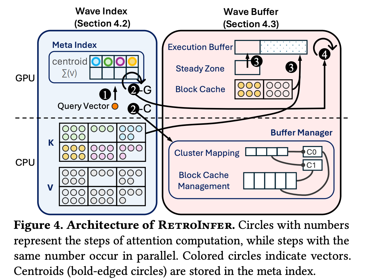
文章由此提出了wave index和wave buffer。

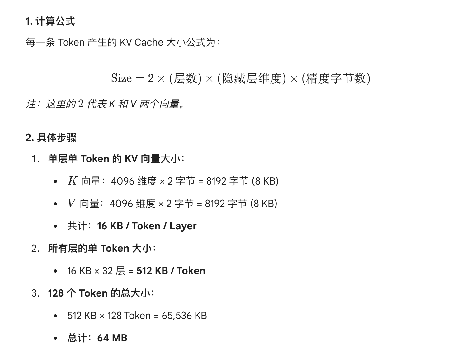
知识回顾：KVCache 计算公式

128个token，在7B模型里可能就要64MB。

一个nb的可视化网站：
https://kvcache.io/

对于一个典型的 7B 模型（以 Llama-2-7B 或 Llama-3-8B 为例），其配置如下：

• 层数 ($L$): 32
• 隐藏层维度 ($d$): 4096
• 注意力头数: 32（如果是全量注意力 MHA，KV 头数也是 32；如果是分组查询注意力 GQA，KV 头数通常更少，这里我们先按标准的 MHA 计算）。
• 精度: FP16（每个参数占 2 字节）。

计算

KV Cache Size = 2 context_length hidden_size (key_value_heads / attention_heads) number_of_layers

重要token是怎么分布的？

首先为什么LLM token分数会分布不均，重点在softmax上，这个指数放大（exponential nature of the softmax function）会很明显。

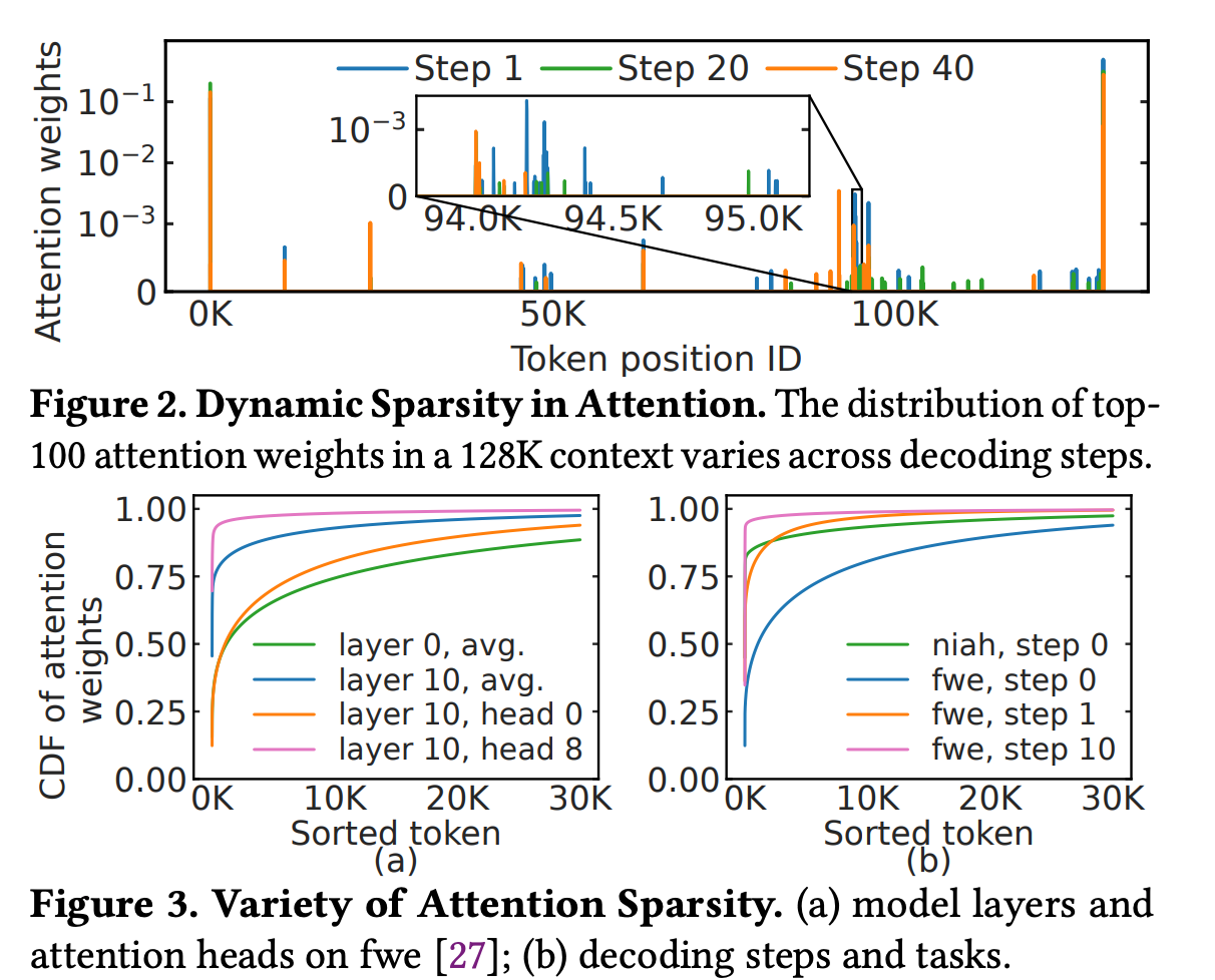
文章提到LLM重要的token的稀疏分布有3个分布特点/难点（这个观察很有趣）：

1. 空间上分布不均。这很好理解，给你一段话，可能重要的词在段首，他们注意力分数高
2. 时间上分布不均，生成token1时的重要注意力和生成token N的重要注意力可能不一样。这个也好理解，比如我们假如喂给GPT两个数学题，GPT在回答第一道题目时，第一题的注意力就高，而回答第二题时，第一题的注意力可能就降下去了。
3. 不同的注意力头，不同的层数里token的分数不同。这个也可以理解。我记得哪篇文章也说过，神经网络就和人脑一样，不同的头会注意句子里的词不同的feature。

下图实验证明了这几点。

The RAG Solution: ANNS

Intro: https://wzbxpy.github.io/LLM-System-and-Engineering/Project-ANNS-and-LLM/ANNS_Introduction.pdf

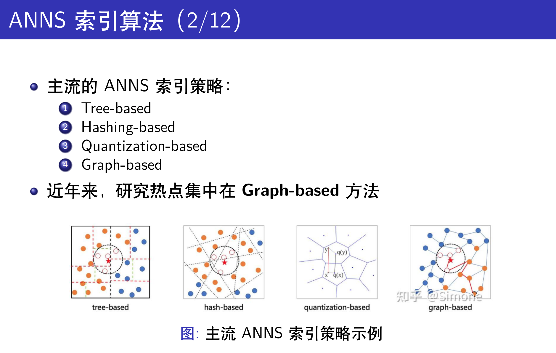
传统ANNS workload：

coarse cluster
  ↓
进几个 cluster
  ↓
取出里面的 vector
  ↓
一个一个算 q·v
  ↓
top-k select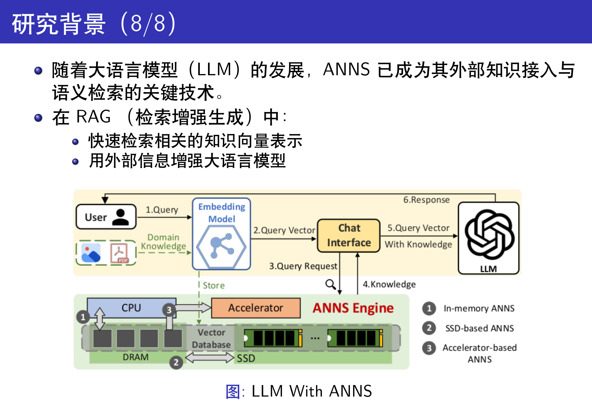

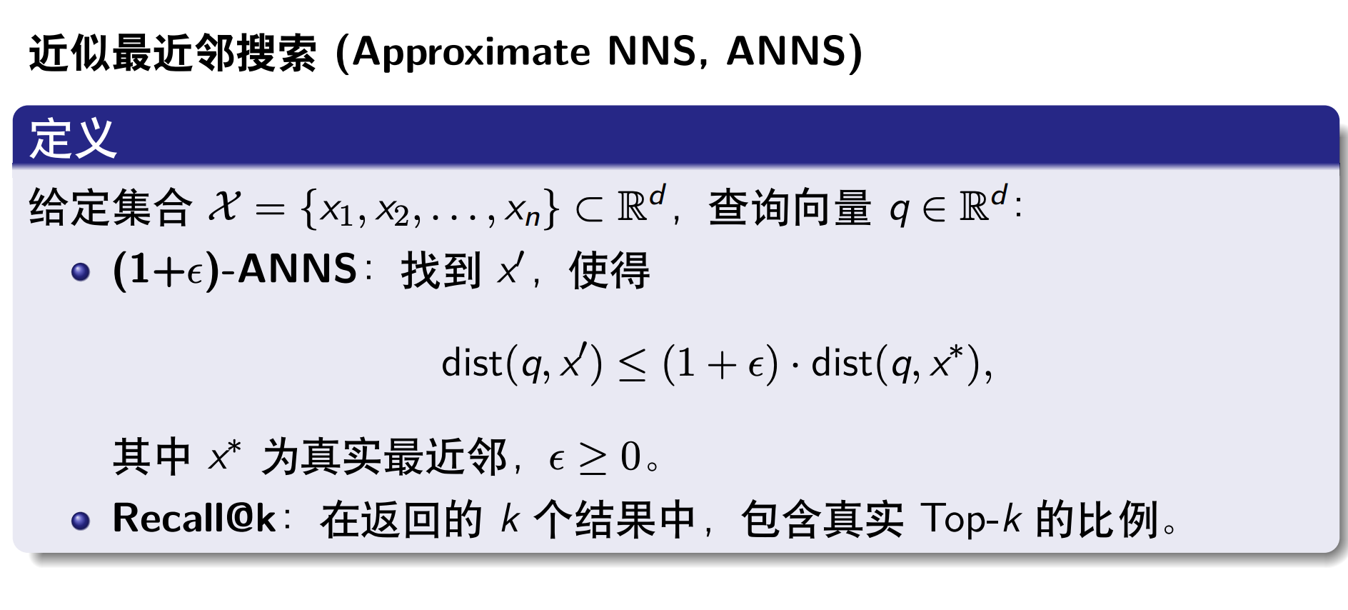
The central research question we address is how to achieve both high accuracy and efficiency in long-context inference. We believe that approximate nearest neighbor search (ANNS) techniques offer a promising path.

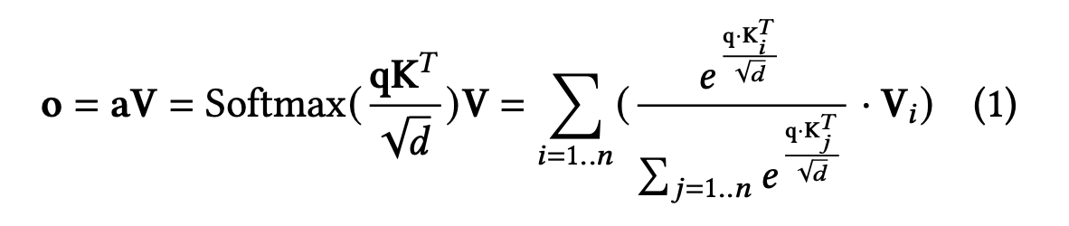
• attention 里本质上是在做 MIPS（Maximum Inner Product Search）：
  对 query 向量 q，找 q·K_i 最大的那些 key
• 这正好是 ANNS 要解决的问题：在高维空间里，近似找 top-k 相似向量
• 于是作者提出：可以把 KV cache 看成一个向量库，用“向量索引”来做 token 选择

ANNS aims to identify a desired number (i.e., top-k) of vectors most similar to a given query in high-dimensional space, using a similarity metric such as inner product. By carefully organizing vectors using a vector index [42, 61], they greatly reduce the number of vectors to access during search while maintaining near-optimal results.

把“attention 的 key 检索”重构成一个“基于聚类的向量索引（wave index）”+ 分区近似计算的系统。

问题：Beyond the accuracy challenges described earlier (§2.3), efficiency challenges arise because incorporating ANNS introduces index traversal and selective data access into an inference system that is otherwise optimized for dense GPU execution

ANNS 不太适合GPU计算：

First, sparse attention with ANNS introduces two types of data (i.e., index structures and KV vectors) and three types of computation (i.e., index traversal, index construction, and attention calculation).

传统 ANNS：选 cluster → 再在 cluster 内选 top-k vector
Wave Index：直接把整个 cluster 的向量都拿来算 attention，避免 GPU 上的 top-k 和随机访存

Second, the system should reduce index traversal and construction costs while preserving retrieval quality. Index traversal on GPUs is costly due to irregular memory accesses and fine-grained operations such as top-k selection. Index construction also introduces non-negligible overhead. These costs can be prohibitive under strict latency constraints.

We advocate building the KV cache as a vector storage system. Such a system leverages a vector-based index to identify important tokens with high quality and incorporates a storage design that comprehensively addresses the accuracy and efficiency challenges discussed above.

Wave index: ANNS for KVCache

Wave index 是一个 cluster-based vector index，灵感来自经典 ANNS，做了三点关键改造

Index Organization: k-means group

1. 用 k-means 聚类所有 key

Wave index partitions the KV vectors in the context into clusters using spherical k-means [26], based on the similarity between key vectors. A centroid is computed as the representative of each cluster–the average of key vectors of one cluster. We observe that the classic cluster-based vector index approach is synergistic with the attention mechanism, because critical key vectors for a given query tend to be grouped within a few clusters, while the critical clusters tend to be irregularly distributed across the context. As illustrated in Figure 5, although several tokens (i.e., 2nd, 4th, and 8th) are irregularly distributed, wave index groups them into the same cluster (i.e., yellow).

token -> groups

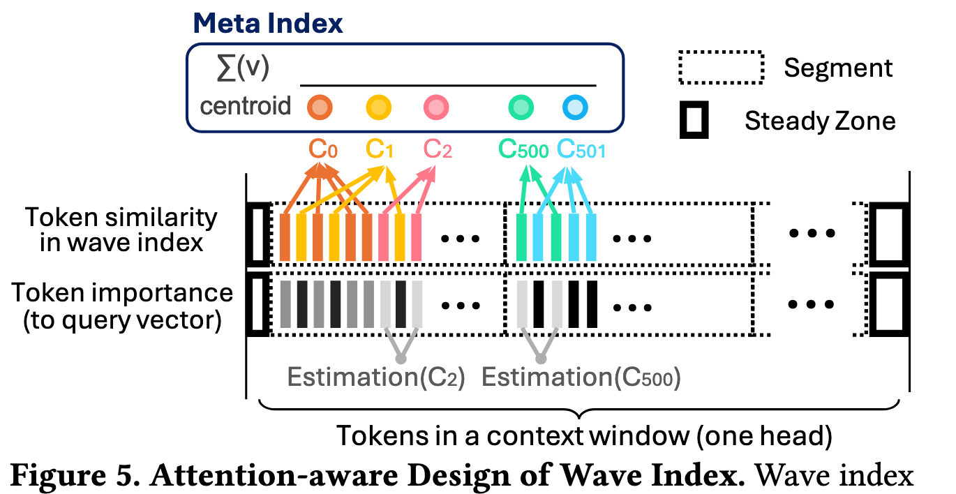
Wave index divides the context into segments (dotted boxes). Each vertical bar represents a token at one position. In the first row, tokens with the same color belong to the same cluster, and similar colors (e.g., yellow and orange) indicate token similarity, which is based on key vector similarity. In the second row, the darker the bar, the more important the token to the query. For example, a query of purple could be close to a red vector (1st segment) and a blue vector (2nd segment).

2. 查询时：不是“找 top-k 向量”，而是“找 top-k cluster”

把 “在几十万 token 里选重要 token” 变成 “在几千个 centroid 里选重要 cluster”
不选top k 向量后，访存会更规则。

文章还解释道：cluster 内向量本来就相似：

Since the clusters are highly coherent, this design also improves the accuracy of attention computation by potentially including more tokens that are also important.

选 cluster
  ↓
整个 cluster 搬过来
  ↓
直接做 attention

However, the goal of classic ANNS is to retrieve the top-k vectors by selecting candidates from clusters and performing pairwise comparisons to the vectors for further ranking, which is costly on GPU. In contrast, wave index retrieves all vectors from the critical clusters and incorporates them directly into the attention computation, avoiding the selection cost.

只做 coarse，不做 fine.
Wave Index：直接把整个 cluster 的所有向量都拿来算 attention，

这样就可以快速计算 哪些 token 要精算，哪些 token 可以“聚合估算

3. Segmented Clustering： 把序列按位置切成段（比如每 8K tokens 一段）， 每一段内部单独 k-means，这样可以提升并行度。

文章提到这样做的理由：RoPE 之后：key 向量在位置上有粗粒度局部性，跨段向量本来就不太相似

To accelerate index construction, we introduce a technique called segmented clustering, where the input sequence is divided into segments, and clustering is performed within each segment, instead of clustering over the entire input sequence as in classic vector index. For example, in Figure 5, vectors in the first segment (i.e., red, yellow, and orange ones) are clustered independently of vectors in the second segment.

To save construction cost, wave index introduces segmented clustering, performing k-means clustering within each segment independently, reducing the time complexity of clustering by a factor of s, where s is the number of segments. This design is based on the observation that key vectors exhibit coarse-grained spatial locality within the input sequence

会影响稀疏吗：

Such coarse-grained spatial locality does not contradict the fact that important tokens (i.e., clusters) are usually scattered throughout the context (Figure 5). This is due to the fact that similarity-based clustering is conducted in a highdimensional vector space and the query vector in attention behaves as a special type of “out-of-distribution query vector.” [39] In this context, the key vectors similar to the query vector can possibly be distant from each other in the vector space [11]. We leverage existing literature [13] to ensure that the clustering effectively captures the attention importance.

Tripartite Attention

wave index把 token 分成三类：

[ Steady Zone | Retrieval Zone | Estimation Zone ]

Steady, Retrieval, and Estimation Zones. Recent studies have revealed that a range of tokens located at the beginning and end of the context are consistently important [74]. These tokens are categorized as steady zone in wave index, as shown in Figure 5. Therefore, tokens in the steady zone are directly included based on their positions, rather than being organized into the vector index. The KV vectors retrieved by the centroids and clusters are categorized as retrieval zone; these tokens are directly used for attention computation.

这里文章一张图介绍了三类token的计算方法。

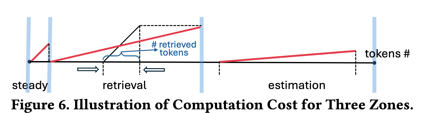
In the steady zone, attention is computed precisely, so the computation cost is linear in the number of tokens (red line’s slope). In the retrieval zone, we calculate attention for the retrieved vectors (whose number is significantly reduced due to sparsity). The computation cost is linear in the number of retrieved vectors (black line), while the overall cost is amortized over the total number of vectors (red line). In the estimation zone, the attention is estimated based on centroids, which incurs a much lower computation cost (red line).

1️⃣ Steady Zone

固定重要 token, 一定要算
经验规律：

• 开头 token
• 最近 window token
  总是重要 → 不走索引，直接全算。

2️⃣ Retrieval Zone

（精算 cluster）
流程：

• 对 query q：
  • 计算：q · centroid_i
  • 排序所有 centroids
  • 选前 r 个 cluster
• 这些 cluster：
  • 把里面所有 K/V 搬到 GPU
  • 做 精确 attention

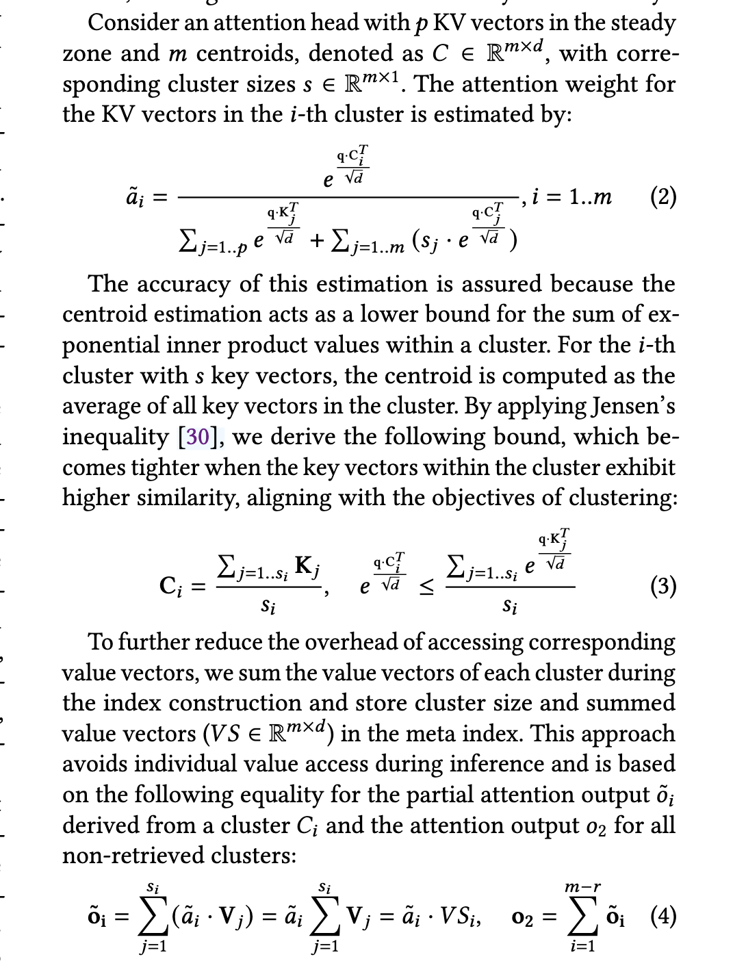
3️⃣ Estimation Zone

（不取 KV，只做估算）
剩下的 cluster 不访问任何真实 K/V！

只用：

• centroid
• cluster size
• sum(V)
  来估算它们对 attention 的贡献。

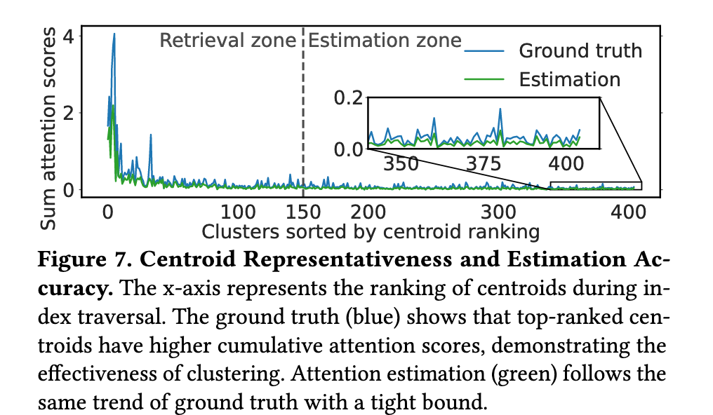
具体操作公式看文章吧，了解思想即可。

流式index更新

不用重新计算 k-means，每次更新计算。经典方法。

During the decoding phase, following segmented clustering, the index is updated incrementally whenever the generated tokens exceeds a segment. we perform k-means clustering only on the newly generated tokens, significantly reducing the index update overhead. This design leverages the coarse-grained spatial locality observed in the generated key vectors, consistent with patterns seen during the prefilling stage. The clustering results from the new segment are appended to the existing index, while the corresponding KV vectors are offloaded to the CPU.

实验证明基本没问题。

计算流程

这样的话，我们的计算为每个 attention head，每一步骤如下：

1. GPU：
   • 计算 q · centroids
   • 排序
2. 分区：
   • steady zone → 已在 GPU
   • retrieval zone → 请求 wave buffer 搬 KV
   • estimation zone → 直接用 meta index 算
3. GPU：
   • FlashAttention 跑 retrieval + steady
   • 同时合并 estimation 的结果

wave buffer

这个工作就很工程了。大概idea是，我们目前已经实现了在CPU上高效读取高attention分数的KVCache，但是，计算没问题了，通信有问题。PCIe带宽不好，GPU内存与CPU内存读取速度不一样。维持，我们可能需要Caching和高效读取。

With the wave index, RetroInfer significantly reduces the number of KV vectors required per query, lowering PCIe traffic to less than 2% of that in full attention. However, the inference throughput could still suffer due to the limited PCIe bandwidth for long-context inference. Drawing on the classic wisdom of computer systems, the performance and capacity disparity between GPU memory and CPU memory, akin to the von Neumann bottleneck [67], necessitates the buffer caches in the fast, low-capacity GPU memory. Thanks to the high-quality retrieval provided by the wave index, adjacent decoding steps for neighboring query vectors show strong temporal locality, as only important tokens are loaded into GPU memory. Thus, caching is highly beneficial.

正如原文说：

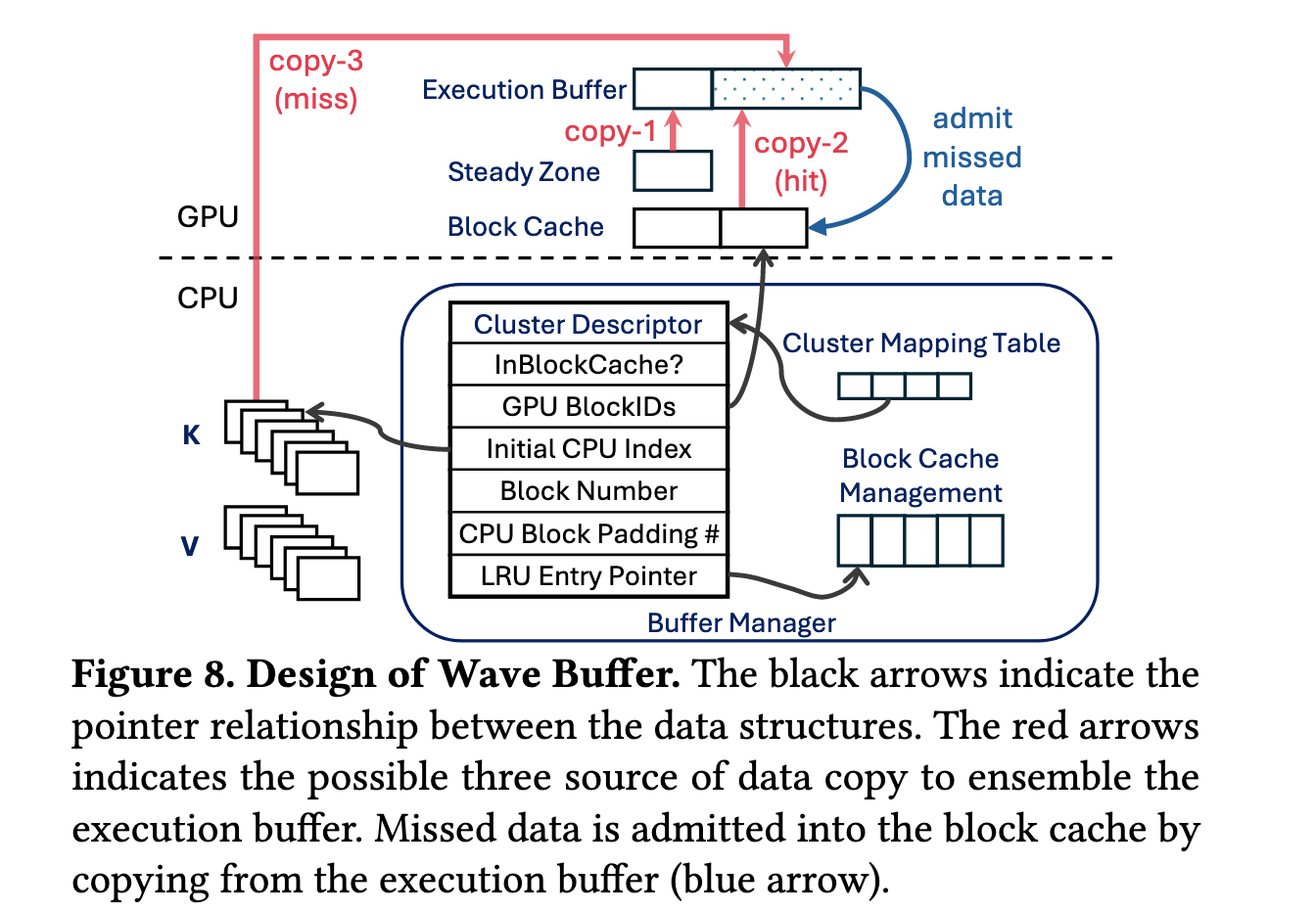
Specifically, what should be cached, how to manage data movement and the control plane of caching, and finally, how can all these movements be effectively parallelized? We address these challenges with the wave buffer, a comprehensive memory management component that aligns well with the attention mechanism.

结构

Buffer Organization：

GPU 上有：

• 🧱 Steady Zone Buffer（小）
• 🧱 KV Block Cache（5% KV，大）
• 🧱 Execution Buffer（每层 attention 用的 staging buffer）

CPU 上有：

• 🧠 Buffer Manager
• 🧠 Cluster Mapping Table（类似页表）
• 🧠 LRU / 替换策略 / block allocator

核心想法是，他们把更新操作和访问操作解偶了。针对访问操作（读取kvcache），他们直接同步开始计算；而针对更新kvcache（与LRU策略等逻辑），是异步CPU-GPU操作。

KVCache Block

5% cache size for KV vectors.

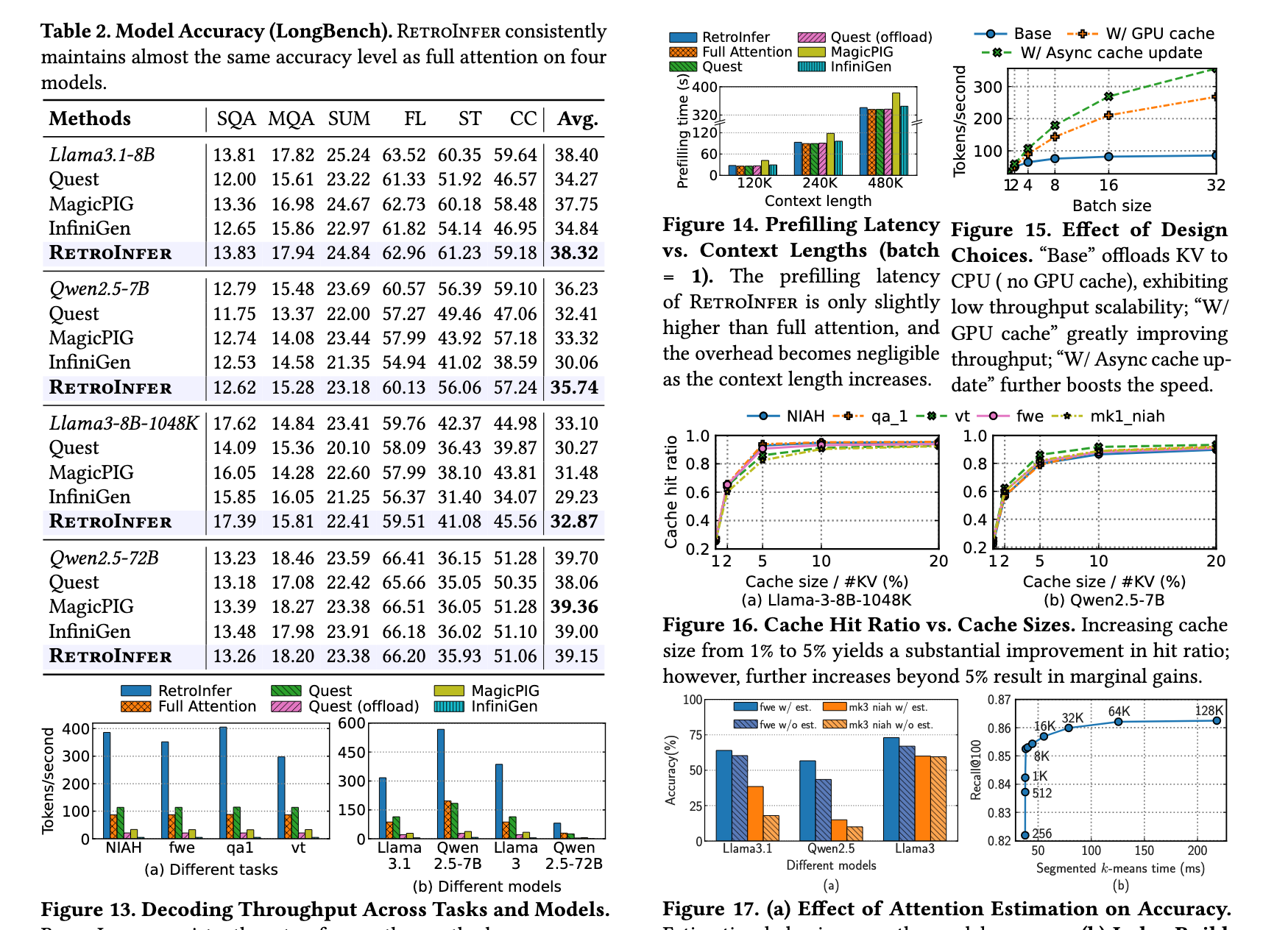
KV Block Cache. We observe a strong temporal locality of important tokens: neighboring decoding steps (i.e., query vectors) have a high overlap of critical tokens due to topic continuity and syntactic proximity. This observation is supported by recent works [70, 75] and an empirical study that examined the cache hit ratio across two models and five tasks (§5.4). With a GPU cache size equal to 5% of the total KV vectors, the average cache hit ratio across tasks ranges from 0.79 to 0.94, indicating high cache-ability of important KV vectors.

Cluster mapping table

Wave index 的单位是cluster，GPU cache 的管理单位是fixed-size block，所以一个 cluster 可能占多个 block，一个 cache miss 要为 cluster 分配多个 block。

上一个这样的需求，是操作系统的页表。因此他们设计了cluster mapping table，每个 entry 记录cluster 是否在GPU以及在CPU、GPU的block位置。

Since the cache replacement logic is relatively complex and difficult to parallelize, we offload it to the CPU. This approach differs from classic caching systems, where the management logic is executed in faster hardware. We use clusters as the cache admission and replacement unit and blocks as the unit for space management. Note that a cluster could be spread across multiple blocks; to admit a missed cluster into the KV block cache, multiple clusters may be evicted until a sufficient number of blocks are freed. We design a cluster mapping table as a layer of indirection. Each entry in the mapping table is a cluster descriptor (Figure 8), mapping a cluster’s addresses in GPU memory and CPU memory, similar in purpose to a page table in operating systems.

The key insight of the wave buffer is to decouple cache access on the critical path from the expensive cache update. This is facilitated by the hybrid GPU+CPU structure–after the lookup, the key-value vectors must be immediately ready for the GPU in the execution buffer, whereas the cache update can be performed asynchronously by the CPU, in parallel with the data copy and attention computation.

Synchronous Cache Access

这一层只做cache访问，不进行cache替换等操作。大概访问过程为：GPU SM -> GPU Cache -> GPU DRAM -> CPU Memory

Upon obtaining the IDs of the clusters in the retrieval zone for a query, the wave index sends these IDs to the CPU thread running the buffer manager, which looks up the mapping table to determine the clusters’ locations and issues the memory copy accordingly.

同步访问：

• Wave index 给出：要用哪些 cluster
• GPU 启动 copy kernel：
  • steady → execution buffer
  • cache hit → execution buffer
  • cache miss → CPU → execution buffer

多线程：

Table lookup is accelerated using CPU multi-threading, without synchronization overhead, as this process is read-only.

Asynchronous Cache Update

CPU收到访问情况后，CPU线程慢慢更新LRU Cache，然后推送到GPU里。

The replacement decision is then enacted by issuing a request to the GPU to schedule a copy from the execution buffer to the block cache, thereby admitting the data into GPU memory and completing the cache update. With the decoupled cache access and update, the latency of CPU involvement is fully overlapped with GPU execution, which accelerates the overall process

Execution buffer

将来路不同的KVCache拼成完整的送给 Flash Attention.

The sequential nature of the execution buffer makes them directly usable by FlashAttention to compute the partial attention output. This output is combined with the estimated attention output in the estimation zone to produce the final attention output.

• steady zone（GPU 上的一小块固定区）
• KV block cache（GPU cache）
• CPU 上的 KV blocks（cache miss）

他们写了一个GPU kernel来同时做三种的copying

Three types of data copy may be needed to assemble the execution buffer, as shown in Figure 8: 1) from the steady zone (GPU to GPU), 2) from the KV block cache (GPU to GPU), and 3) from KV blocks (CPU to GPU). We have developed a highly-optimized copy operator, which enables parallel execution of three types of data copying, each accelerated using numerous GPU threads (details in §4.5).

Constrain Prefilling Latency

大概就是流水的去做Prefill

不流水做法：

GPU: 算 QKV
CPU: 等
GPU: 做 clustering
CPU: 再建 mapping table
GPU: 等
CPU: 再拷 KV

CPU-GPU pipeline:

GPU:
  - 一边算 QKV
  - 一边跑 segmented clustering

CPU:
  - 一边接收 KV
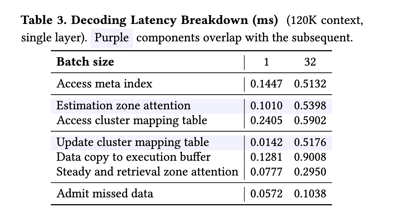
  - 一边建 mapping table / cache metadata

We carefully constrain prefilling latency by fully utilizing GPU–CPU parallelism. After obtaining the Q, K, and V during prefilling, RetroInfer asynchronously offloads the KV vectors to CPU memory while the GPU performs segmented clustering. The clustering results are then sent to the CPU, allowing the wave buffer to construct its data structures, including the mapping table and metadata for cache replacement. With this parallelism, only segmented clustering remains on the critical path of the prefilling phase, and its latency is negligible (less than 5%, as shown in §5).

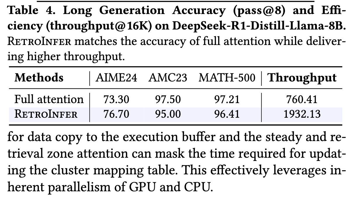
Impl & Exp & Related works

We implement CUDA kernels (~1,000 LoC) to support execution buffer transfers and block cache updates

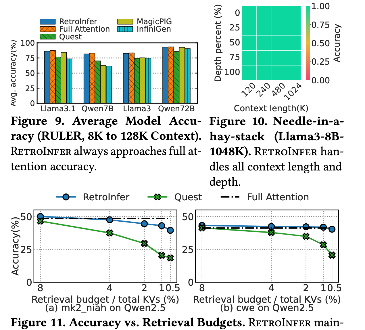
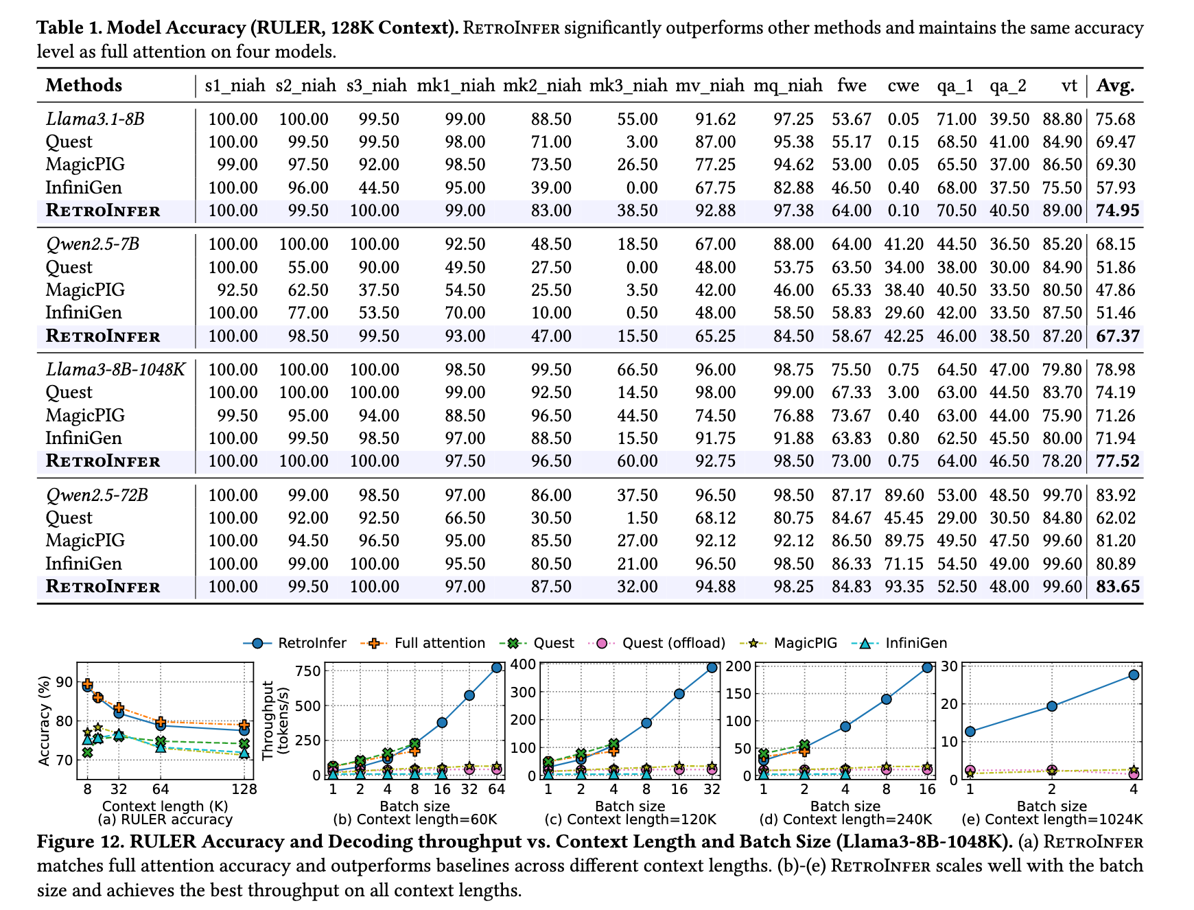
可以看到得分是比原模型低了些，但是总体还挺高。然后速度快了很多。

LLM Serving Systems. Recent research has explored various strategies for LLM serving efficiency [3, 15, 32, 37, 58, 64, 79, 86, 87]. LoongServe [69] proposes an elastic sequence parallelism scheduling algorithm for long-context requests. Many works [12, 16, 17, 52, 80] also offload KV caches to CPU or disk to alleviate the memory capacity limit. These works focus on different aspects of long-context serving and are complementary to RetroInfer.

Sparse Attention. To accelerate long-context inference, many works exploit attention sparsity. Static sparsity methods [35, 73, 74] maintain fixed patterns during decoding but compromise model accuracy. Many dynamic sparsity methods [13, 33, 65, 72, 77, 82, 84] heuristically select KV pairs per step. Recent works [24, 39] also explore leveraging vector indexes for KV cache retrieval. However, they are limited to prefix caching or offline inference scenarios due to the high cost of index construction. PyramidKV [9] and D2O [68] adapt retrieval budgets across layers but do not consider sparsity variation across queries and tasks. Tactic [88], a concurrent effort, adjusts budgets via distribution fitting, though its accuracy and efficiency depend on fitting precision. Our work also focuses more on system-level design than on pure algorithmic improvements. Some sparse attention approaches [18, 81] require costly model retraining to learn dynamic sparsity. Other techniques include scalar KV cache quantization [25, 40, 83] and sparsity for accelerating prefilling [31], both of which are complementary to our work.

LLM Weight Sparsity. Model weight compression and offloading techniques [5, 38, 59, 62, 76, 85] enable LLMs to run on memory-constrained devices. These are orthogonal to RetroInfer, which targets scenarios where the KV cache, not the weights, is the memory bottleneck.