DnCC3: Introduction to Spark

In this assignment, we need to use Spark to analyze the Parking dataset.

Preparing

Install pysark and java

pip install pyspark
sudo apt-get update
sudo apt-get install openjdk-17-jdk
export JAVA_HOME=/usr/lib/jvm/java-17-openjdk-amd64
export PATH=$JAVA_HOME/bin:$PATH

Init Spark:

from pyspark.sql import SparkSession
import os

# java env
os.environ["JAVA_HOME"] = "/usr/lib/jvm/java-17-openjdk-amd64"

spark = SparkSession.builder.appName("A3").getOrCreate()
print(spark)

Sava as CSV:

import shutil
import os

def save_as_single_csv(df, output_filename):
    tmp_dir = output_filename + "_tmp"

    # 1. Coalesce to 1 partition → ensures only 1 part file
    df.coalesce(1).write.csv(tmp_dir, header=True, mode="overwrite")
    # 2. Find generated part file
    part_file = None
    for f in os.listdir(tmp_dir):
        if f.startswith("part-") and f.endswith(".csv"):
            part_file = f
            break
    # 3. Move and rename to desired output filename
    shutil.move(os.path.join(tmp_dir, part_file), output_filename)
    # 4. Delete temp directory
    shutil.rmtree(tmp_dir)

PySpark calls used:

• coalesce(1).write.csv("r2.csv", header=True, mode="overwrite")
  to output a single CSV file.

Task1: berthagesfor number in each section

from pyspark.sql import SparkSession
from pyspark.sql.functions import countDistinct

df = spark.read.csv("parking_data_sz.csv", header=True)
# Task 1
r1 = df.groupBy("section") \
       .agg(countDistinct("berthage").alias("count"))

To compute the number of unique berthages in each section, I loaded the CSV into a Spark DataFrame and applied a groupBy("section") followed by countDistinct("berthage"). This efficiently aggregates the dataset in parallel and ensures that duplicated berthagesfor entries are not counted.

PySpark calls used:

• spark.read.csv("parking_data_sz.csv", header=True)
  to load the CSV dataset as a DataFrame.
• groupBy("section")
  to aggregate rows by section.
• countDistinct("berthage")
  to count unique berth IDs per section.
• alias("count")
  to rename the aggregated column to count.

Task2: berthagesfor in each section

from pyspark.sql import SparkSession
from pyspark.sql.functions import col

df = spark.read.csv("parking_data_sz.csv", header=True)

# Task 2
r2 = df.select("berthage", "section").distinct()

To list all unique berthage–section pairs, I selected the berthage and section columns from the DataFrame and applied distinct(). This removes duplicate rows in the raw data and produces a clean mapping showing which berthages belong to which sections.

PySpark calls used:

• select("berthage", "section")
  to project only the relevant columns
• distinct()
  to remove duplicate (berthage, section) pairs.

Task3: Average parking time for each section

from pyspark.sql.functions import unix_timestamp, avg

# Filter invalid rows
df_valid = df.filter(unix_timestamp("out_time") > unix_timestamp("in_time"))

# Compute parking time in seconds
df_time = df_valid.withColumn(
    "parking_seconds",
    unix_timestamp("out_time") - unix_timestamp("in_time")
)

# Task 3: avg parking time per section
r3 = df_time.groupBy("section") \
            .agg(avg("parking_seconds").cast("int").alias("avg_parking_time"))

To compute the average parking duration for each section, I first use filter filtered out records where the out_time is earlier than the in_time.

Then, I calculated each vehicle’s parking time by subtracting the corresponding timestamps.

After adding this duration as a new column, I grouped the data by section and applied avg() to obtain the mean parking time in seconds for each section.

PySpark calls used.

• to_timestamp("in_time"), to_timestamp("out_time")
  (or unix_timestamp) to parse the time strings into timestamps.
• filter(unix_timestamp("out_time") > unix_timestamp("in_time"))
  to remove invalid rows.
• withColumn("parking_seconds", unix_timestamp("out_time") - unix_timestamp("in_time"))
  to compute per-record parking duration.
• groupBy("section").agg(avg("parking_seconds").cast("int").alias("avg_parking_time"))
  to compute integer average parking time per section.

Task4: Average parking time for each berthage in descending order

# Task 4: avg parking time per berthage
r4 = df_time.groupBy("berthage") \
            .agg(avg("parking_seconds").cast("int").alias("avg_parking_time")) \
            .orderBy(col("avg_parking_time").desc())

To compute the average parking time for each berthage, I grouped the preprocessed DataFrame by berthage and applied avg() on the computed parking duration column. The resulting averages were then sorted in descending order by avg_parking_time to highlight berthages with the longest typical parking times.

PySpark calls used.

• groupBy("berthage")
  to aggregate durations by berthage.
• agg(avg("parking_seconds").cast("int").alias("avg_parking_time"))
  to compute integer average parking time per berth.
• orderBy(col("avg_parking_time").desc())
  to sort in descending order of average duration.

Task5: Average berthages usage of each section

For each section, output the total number of berthages in use and the percentage of in-use berthages in that section, in a one-hour interval (e.g. during 09:00:00-10:00:00). “In use” means there is at least one vehicle parked in that berthage in that interval for ANY duration. The time intervals should begin at the start of the first hour that appears in the dataset (for example, if the first entry is at 12:23, the first interval should start from 12:00). The output file should have the columns start_time, end_time, section, count and percentage. The percentage value should be rounded to one decimal place (e.g. 67.8%). The data format of start_time and end_time should match the one in the original dataset “YYYY-MM-DD HH:MM:SS”.

from pyspark.sql import SparkSession
from pyspark.sql.functions import (
    to_timestamp, unix_timestamp, date_trunc, sequence, explode,
    countDistinct, count, col, expr, round, concat, lit, date_format
)

# 1. Filter invalid rows
df_ts = df.withColumn("in_ts",  to_timestamp("in_time")) \
          .withColumn("out_ts", to_timestamp("out_time"))

df_valid = df_ts.filter(col("out_ts") > col("in_ts"))

# 2. preprocess time, construct all full hour_start covered by [in_ts, out_ts)
#    To avoid counting the hour that is exactly the out_ts, use out_ts - 1 SECOND
df_valid = df_valid.withColumn("out_adj", expr("out_ts - INTERVAL 1 SECOND"))

# Each record's first and last hour_start (truncated to hour)
df_valid = df_valid.withColumn("start_hour", date_trunc("hour", col("in_ts"))) \
                   .withColumn("end_hour",   date_trunc("hour", col("out_adj")))

# Generate array of hour_start timestamps covered by [start_hour, end_hour]
df_valid = df_valid.withColumn(
    "hour_start_array",
    sequence(col("start_hour"), col("end_hour"), expr("INTERVAL 1 HOUR"))
)

# Expand into multiple rows: each row is a (section, berthage, hour_start)
df_expanded = df_valid.select(
    "section",
    "berthage",
    explode(col("hour_start_array")).alias("hour_start")
)

# 3. Calculate total berthage count for each section (global, not time-specific)
section_total = df.select("section", "berthage") \
                  .distinct() \
                  .groupBy("section") \
                  .agg(count("berthage").alias("total_berthages"))

# 4. Calculate the number of "in use" berthages (distinct) for each (section, hour_start)
in_use = df_expanded.groupBy("section", "hour_start") \
                    .agg(countDistinct("berthage").alias("count"))

# 5. Calculate percentage + add start_time / end_time fields
r5 = in_use.join(section_total, on="section", how="left")

r5 = r5.withColumn(
        "percentage_num",
        round(col("count") * 100.0 / col("total_berthages"), 1)
    ) \
    .withColumn(
        "percentage",
        concat(col("percentage_num").cast("string"), lit("%"))
    ) \
    .withColumn(
        "start_time",
        date_format(col("hour_start"), "yyyy-MM-dd HH:mm:ss")
    ) \
    .withColumn(
        "end_time",
        date_format(expr("hour_start + INTERVAL 1 HOUR"), "yyyy-MM-dd HH:mm:ss")
    ) \
    .select(
        "start_time",
        "end_time",
        "section",
        "count",
        "percentage"
    ) \
    .orderBy("start_time", "section")

To compute the hourly berthage usage for each section, I first preprocessed the dataset by converting the in_time and out_time fields into timestamp columns and filtering out invalid rows where the departure time is earlier than the arrival time.

Because the task requires determining whether a berthage is “in use” during any portion of a given hour, I expanded each parking interval into the list of hour-aligned timestamps it overlaps. Specifically, for every record, I truncated both the entry and adjusted exit times to the nearest hour and generated a sequence of hourly boundaries between them. Exploding this sequence allowed each vehicle to contribute one row per hour in which it was present.

Next, I counted the number of distinct berthages in use for every (section, hour_start) pair. In parallel, I computed the total number of berthages in each section by taking the distinct (section, berthage) combinations in the dataset. Joining these results enabled calculation of the usage percentage per hour as the ratio of occupied berthages to total berthages in that section, rounded to one decimal place as required.

Finally, I formatted each hourly window using start_time and end_time fields matching the dataset’s timestamp style (YYYY-MM-DD HH:MM:SS) and ordered all records by time and section. The final output includes the columns start_time, end_time, section, count, and percentage, providing a clear summary of hourly berthage utilization across all sections.

PySpark calls used.

• withColumn("in_ts", to_timestamp("in_time")), withColumn("out_ts", to_timestamp("out_time"))
  to create timestamp columns.
• filter(col("out_ts") > col("in_ts"))
  to exclude invalid records.
• withColumn("out_adj", expr("out_ts - INTERVAL 1 SECOND"))
  to avoid counting records exactly at the hour boundary in the next interval.
• date_trunc("hour", col("in_ts")), date_trunc("hour", col("out_adj"))
  to align times to the beginning of hours.
• sequence(col("start_hour"), col("end_hour"), expr("INTERVAL 1 HOUR"))
  to generate all hour starts covered by each record.
• explode("hour_start_array")
  to turn each array of hour starts into multiple rows.
• distinct(), groupBy("section").agg(count("berthage").alias("total_berthages"))
  to compute the total number of berthages per section.
• groupBy("section", "hour_start").agg(countDistinct("berthage").alias("count"))
  to count in-use berthages for each section–hour pair.
• join(section_total, on="section", how="left")
  to join in the total berthages.
• round(col("count") * 100.0 / col("total_berthages"), 1)
  to compute the percentage.
• concat(col("percentage_num").cast("string"), lit("%"))
  to format the percentage with a % sign.
• date_format(col("hour_start"), "yyyy-MM-dd HH:mm:ss") and expr("hour_start + INTERVAL 1 HOUR")
  to build start_time and end_time strings.
• orderBy("start_time", "section")
  to sort the output.

Parking Analysis

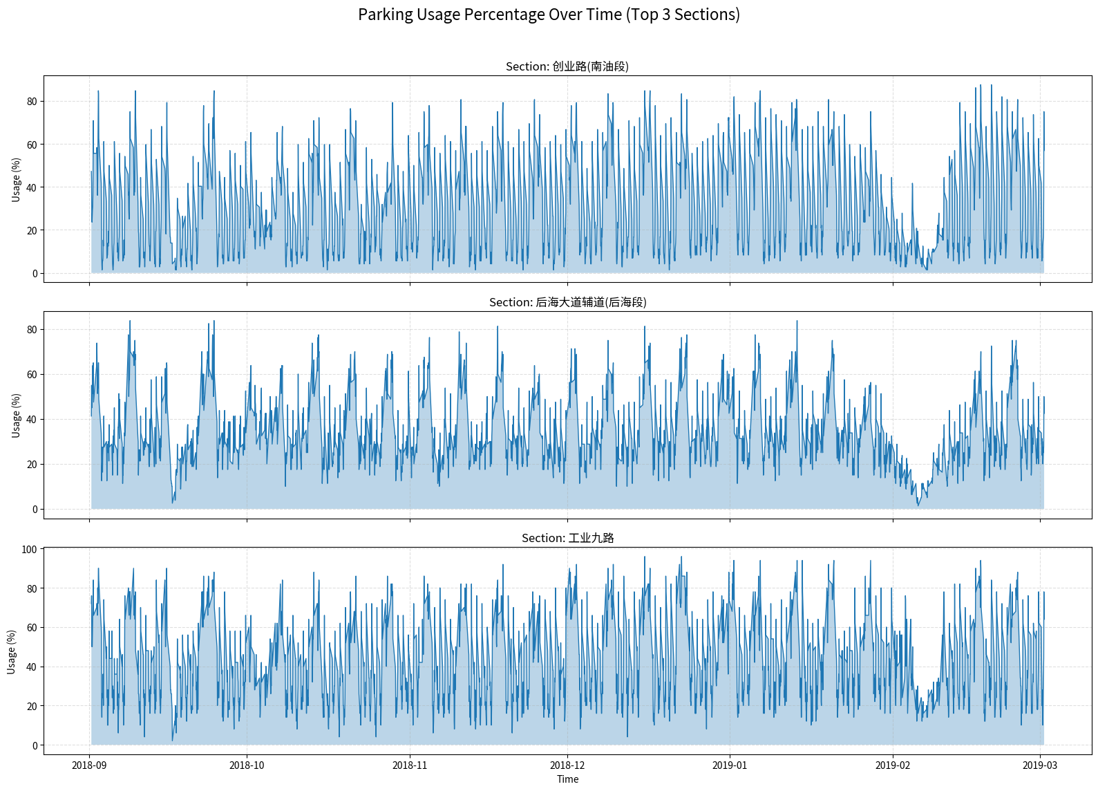
We select the top 3 most frequent sections to do analysis:

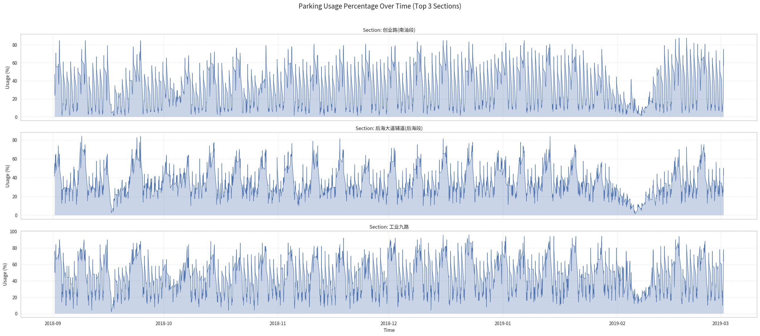
Here we can see 3 trend:

Daily (Diurnal) Parking Patterns

The plots show a clear daily cycle in parking usage. Some sections experience higher occupancy during daytime and lower usage at night, indicating areas dominated by commercial or office activity. Other sections exhibit the opposite trend, with high nighttime usage and lower daytime demand, reflecting residential zones where cars return in the evening.

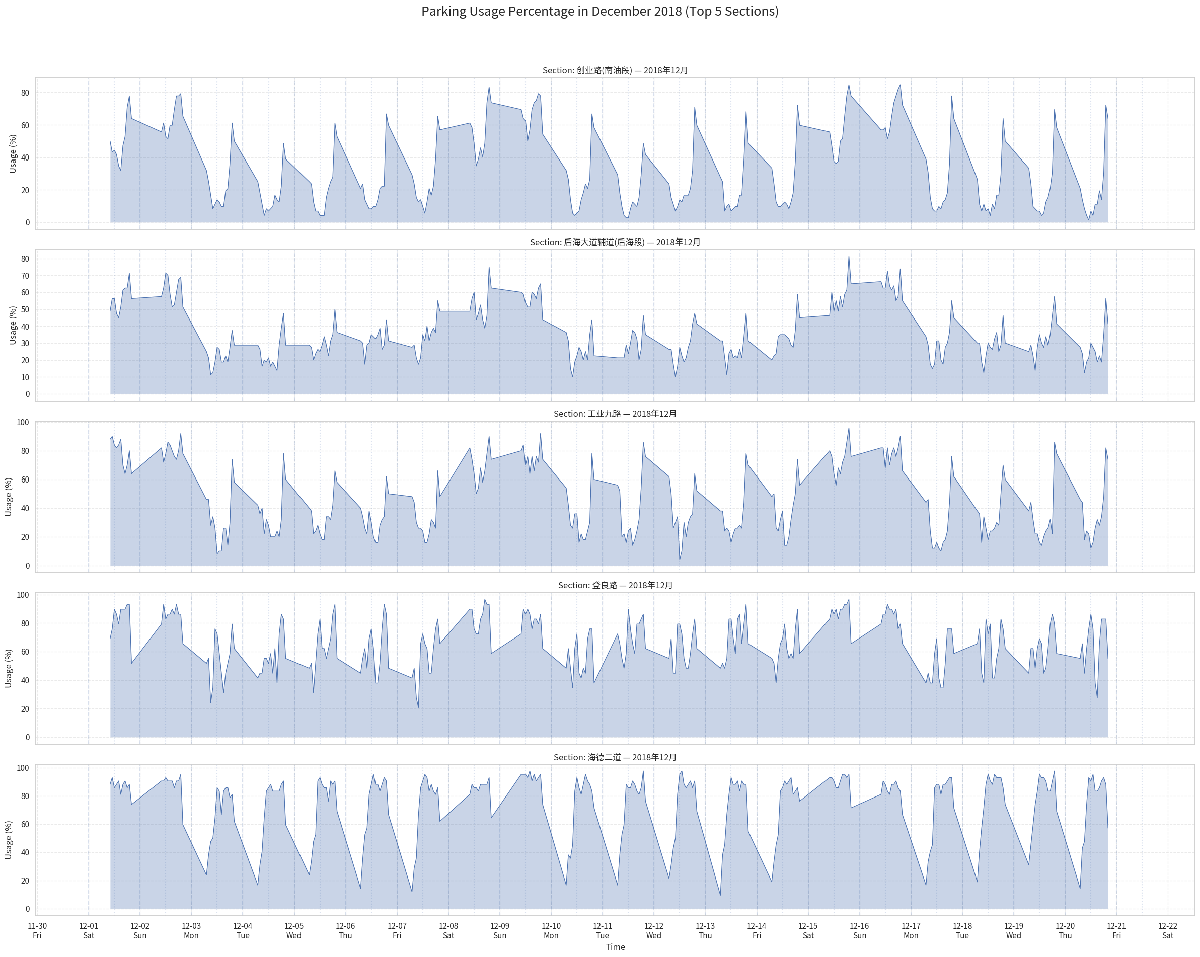
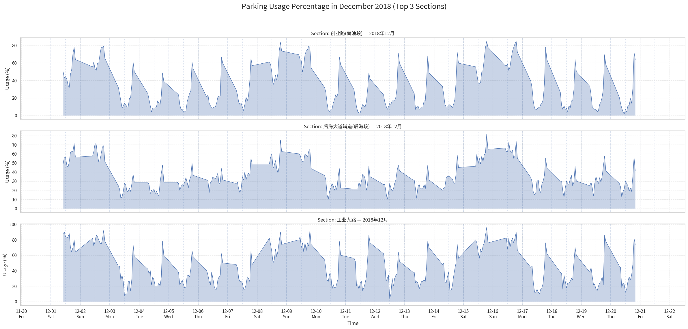
The December plots reveal that different sections exhibit distinct daily parking behaviors.

Let's take 2 roads as examples.

Chuangye Road 创业路（南油段）(the first chart) shows a pronounced midday dip: usage drops significantly around noon each day before rising again in the evening. This pattern is characteristic of areas where vehicles leave during daytime—likely due to commuters driving away for work or business—resulting in relatively low occupancy around noon.

In contrast, Haide Street 海德二道 (the No.5 chart) displays the opposite trend. Its usage peaks around midday and remains relatively high throughout the daytime hours. Such behavior suggests that this area functions as a commercial or office zone where vehicles arrive in the morning and stay parked during working hours, leading to higher occupancy around noon. Usage then decreases noticeably in the evening as vehicles leave the area.

These contrasting patterns highlight how parking data reflects the functional differences between neighborhoods: 创业路 behaves more like a residential zone, while 海德二道 aligns with daytime commercial activity.

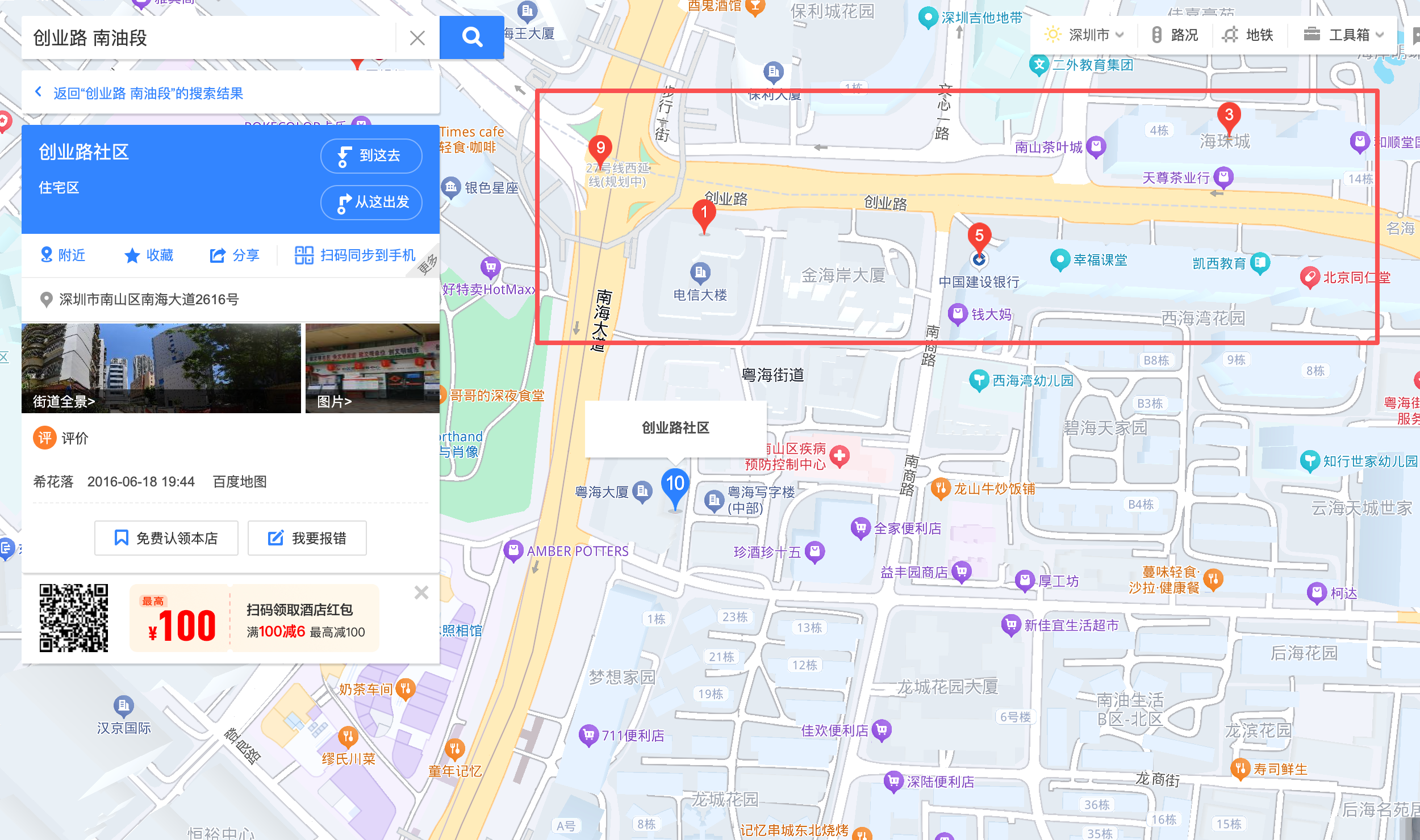
创业路 Chuangye Road Landscape

It looks like some place to live.

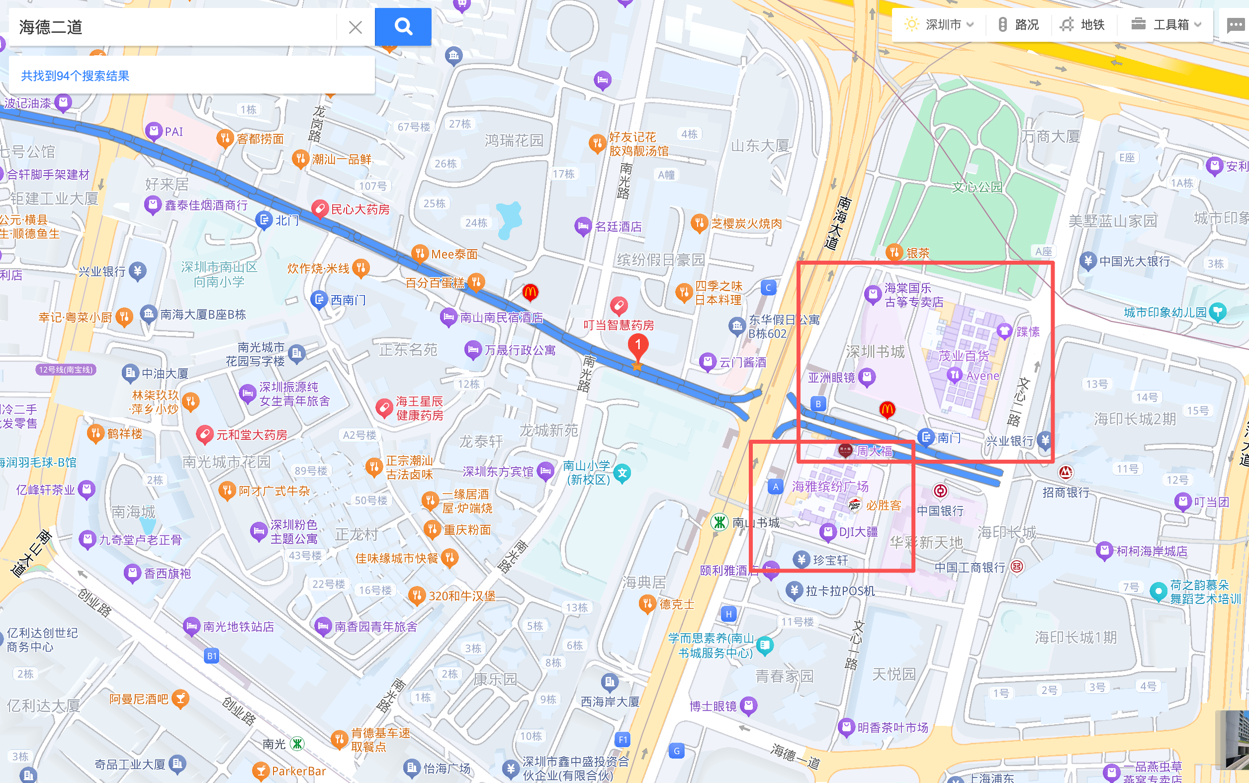
海德二道 Haide Street Landscape
We got Shenzhen bookstore 深圳书城 and several big stores here.

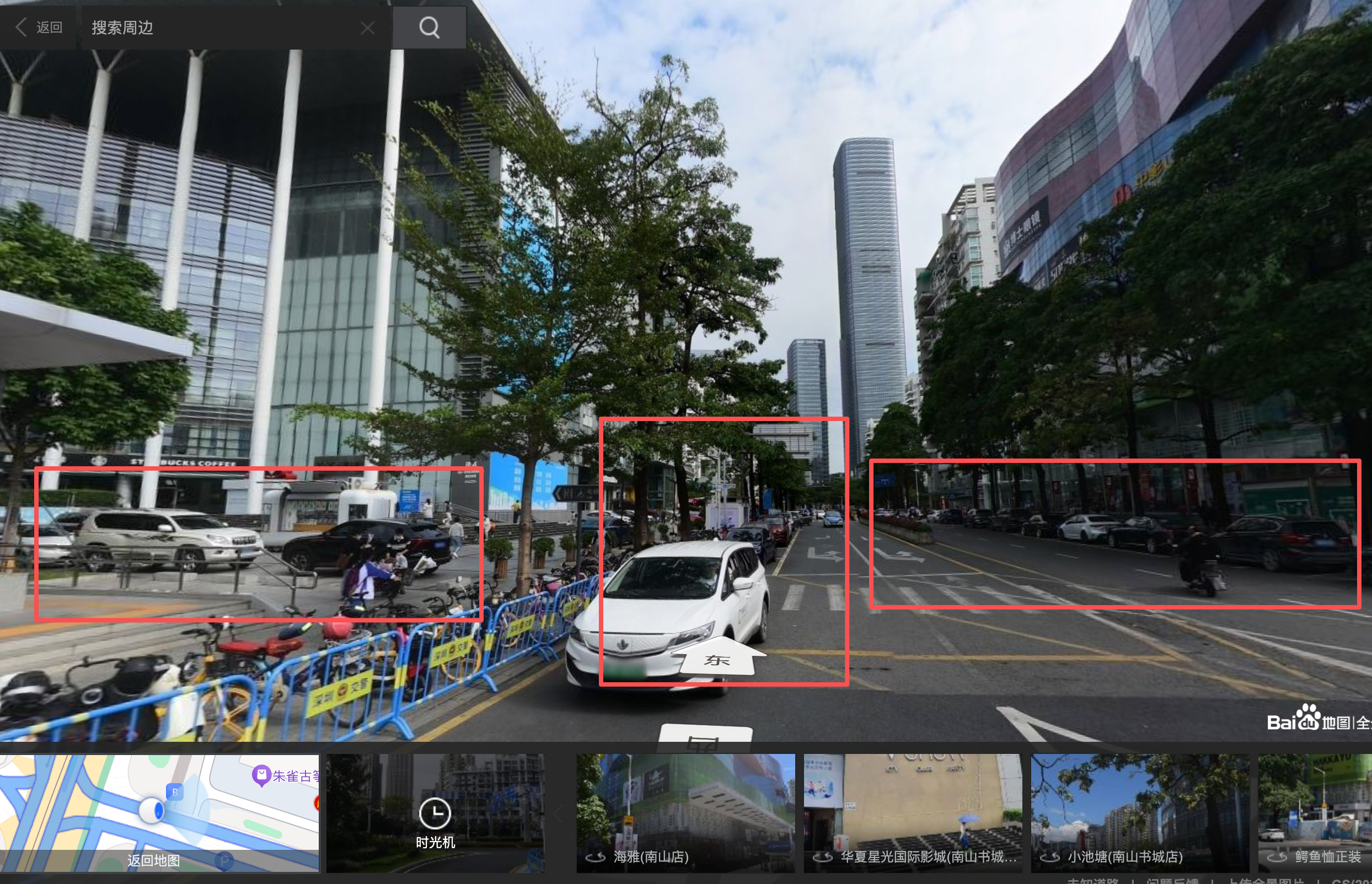
That's why it has high parking utilization during daytime.

Weekly Variation: Weekdays vs. Weekends

A consistent weekly pattern is also visible: parking usage tends to increase on weekends and decrease on weekdays. This suggests different behavioral patterns between workdays—when many vehicles leave for commuting—and weekends, when residents stay nearby and overall parking occupancy rises.

Holiday Effect: Chinese New Year (February 2018)

Around February 5th, 2018—the period of the Chinese New Year—the usage across all sections drops sharply and remains low for several days. This corresponds to the nationwide travel season when many people return to their hometowns, resulting in significantly reduced parking demand throughout the city.

The drawing code (not completed):

# 1. Read data
df = pd.read_csv("r5.csv")
df["percentage"] = df["percentage"].str.replace("%", "").astype(float)
df["start_time"] = pd.to_datetime(df["start_time"])

# 2. Select the top 3 most frequent sections
top_sections = (
    df["section"]
    .value_counts()
    .head(3)
    .index
    .tolist()
)

df_sel = df[df["section"].isin(top_sections)]
df_sel = df_sel.sort_values(["section", "start_time"])

# 3. Plot three subplots
fig, axes = plt.subplots(nrows=3, ncols=1, figsize=(16, 12), sharex=True)

if isinstance(axes, np.ndarray):
    axes = axes.flatten().tolist()
else:
    axes = [axes]

for ax, sec in zip(axes, top_sections):
    sub = df_sel[df_sel["section"] == sec]

    ax.plot(sub["start_time"], sub["percentage"], linewidth=1)
    ax.fill_between(sub["start_time"], sub["percentage"], alpha=0.3)

    ax.set_ylabel("Usage (%)")
    ax.set_title(f"Section: {sec}")
    ax.grid(True, linestyle="--", alpha=0.4)

axes[-1].set_xlabel("Time")

plt.show()

import pandas as pd
import matplotlib.pyplot as plt
import numpy as np
import matplotlib.font_manager as fm
import matplotlib.dates as mdates

# -------- 字体设置 --------
font_path = "/home/haibin/distributed_system/assignment3/static/NotoSansSC-Regular.ttf"
fm.fontManager.addfont(font_path)
plt.rcParams["font.family"] = "Noto Sans SC"
plt.rcParams["axes.unicode_minus"] = False
# --------------------------

# 1. Load data
df = pd.read_csv("r5.csv")
df["percentage"] = df["percentage"].str.replace("%", "").astype(float)
df["start_time"] = pd.to_datetime(df["start_time"])

number = 5

# 2. 选择 12 月最常出现的 3 个 section
top_sections = (
    df["section"]
    .value_counts()
    .head(number)
    .index
    .tolist()
)

# 3. 只保留 2018-12 的数据
df_dec = df[
    (df["start_time"] >= "2018-12-01") &
    (df["start_time"] <  "2018-12-21")
]

df_sel = df_dec[df_dec["section"].isin(top_sections)]
df_sel = df_sel.sort_values(["section", "start_time"])

# 4. 创建子图
fig, axes = plt.subplots(nrows=number, ncols=1, figsize=(24, number * 4), sharex=True)

if isinstance(axes, np.ndarray):
    axes = axes.flatten().tolist()
else:
    axes = [axes]

# ====== 预先算好每天的 0:00 和 12:00 ======
# 所有日期（按天归一化）
all_days = pd.date_range("2018-12-01", "2018-12-21", freq="D")
midnights = all_days                # 每天 00:00
noons = all_days + pd.Timedelta(hours=12)  # 每天 12:00
# ======================================

for ax, sec in zip(axes, top_sections):
    sub = df_sel[df_sel["section"] == sec]

    # 曲线 + 面积
    ax.plot(sub["start_time"], sub["percentage"], linewidth=1)
    ax.fill_between(sub["start_time"], sub["percentage"], alpha=0.3)

    # 画每天 0:00 的竖线（虚线），用来分隔日期
    for t in midnights:
        ax.axvline(t, linestyle="--", alpha=0.2)

    # 画每天 12:00 的竖线（点划线）
    for t in noons:
        ax.axvline(t, linestyle=":", alpha=0.2)

    ax.set_ylabel("Usage (%)")
    ax.set_title(f"Section: {sec} — 2018年12月")
    ax.grid(True, linestyle="--", alpha=0.4)

# X 轴：日期 + 星期几，比如 12-01\nSat
locator = mdates.DayLocator(interval=1)  # 每天一个刻度
formatter = mdates.DateFormatter("%m-%d\n%a")  # 月-日 + 星期（Mon/Tue/...）

for ax in axes:
    ax.xaxis.set_major_locator(locator)
    ax.xaxis.set_major_formatter(formatter)

axes[-1].set_xlabel("Time")

fig.suptitle(f"Parking Usage Percentage in December 2018 (Top {number} Sections)", fontsize=18)
plt.tight_layout(rect=[0, 0.03, 1, 0.95])
plt.show()